

Three ways to study the same subject: a full, paced explanation; a self-contained rapid revision handbook; and questions with concealed answers.
| Part | What you will find |
|---|---|
| I. Detailed understanding | Definitions, worked calculations, diagrams, operational tradeoffs and practice prompts. |
| II. Rapid revision | A separate concise reading sequence with its own explanations, comparison tables, examples, and topic navigation. |
| III. Questions and answers | Questions across the full subject, concealed answers, applied scenarios, and optional calculation and debugging exercises. |
Choose the part for your current task. Within rapid revision, the topic links stay in that section.
Part I — Detailed understanding
A large language model (LLM) is a neural network trained on large amounts of language data to model language and perform tasks such as text generation and understanding. Its parameters are numerical values learned during training. There is no universal parameter-count threshold that makes a model “large.”
This chapter follows an autoregressive, decoder-only Transformer: it predicts a probability distribution over the next token, selects a token, and repeats using the growing sequence. That is the scope of the generation examples, not the definition of every language model. Encoder models, encoder–decoder models and hybrid architectures appear later with their own information flow.
Start with the standard definitions
| Term | Definition | Concrete example and lesson |
|---|---|---|
| Language model | A model of probabilities over language sequences or their constituent tokens, according to its training objective. | A causal model estimates P(sat | The cat). Prediction. |
| Token | A discrete unit represented by an ID in a model's vocabulary. | A word can span several subword tokens. Tokenization. |
| Embedding | A vector representation of an item; a token embedding is the learned vector selected by its token ID. | ID 2 selects row 2 rather than multiplying that row by 2. Representations. |
| Self-attention | Attention whose queries, keys and values come from the same sequence of representations. | A position combines allowed source value vectors using query–key scores. Attention. |
| Transformer | A neural-network architecture using attention and position-wise feed-forward transformations, with residual connections and normalization. | Follow one complete block and its tensor shapes in section 16. |
| Training | Optimizing trainable parameters using data and an objective. | Calculate cross-entropy, backpropagate gradients, apply an optimizer update. Training. |
| Inference | Computing model outputs using learned parameters. | A changed prompt changes activations while ordinary inference keeps parameters fixed. Prefill and decode. |
Technical example: given The backup is stored in the archive. Where is the backup stored?, a supported response is In the archive. We use this short evidence-based question to track changes to the prompt and generated sequence. The separate The cat sat examples isolate matrix arithmetic. All hand-chosen vectors, probabilities and workload figures are teaching assumptions, not measurements from a commercial model.
The six learning objectives are:
- Convert text into token IDs and vectors.
- Calculate how allowed positions contribute through attention.
- Assemble the complete Transformer and output-selection path.
- Derive a training loss and parameter update.
- Estimate serving memory, latency and cost.
- Defend an application decision using quality and operational evidence.
Choose a route and a stopping point
You need ordinary arithmetic and the idea of a percentage to start. When a new kind of calculation is needed, we will explain its purpose and work an example before using the compact mathematical notation. Our main example writes from left to right: it chooses the next token using the input and the tokens it has already generated. The technical name for this design is a causal decoder. Here, “causal” means that a calculation for a token position can use that token and earlier text, but cannot look ahead to later text. “Decoder” refers to the part that produces the output. Section 17 compares it with other designs.
Use these six stages to organize your study. A stage can take several sittings, especially when the mathematics or programming is new. At each stopping point, close the explanation and do the check aloud. Move on when you can explain the steps, rather than when a timer expires.
| Study stage | Read | Ready to continue when you can… |
|---|---|---|
| Represent the text | Sections 1–6 | Explain which numbers identify text, which numbers training changes, and which numbers are calculated for this request. |
| Move information between positions | Sections 7–13 | Calculate how three positions contribute to one result and show which positions are allowed to contribute. |
| Assemble a model | Sections 14–18 | Follow a token’s representation vector through the model to the selection of the next token. |
| Learn the weights | Sections 19–21 | Follow one change to a model parameter and explain how to check whether that change helps on new examples. |
| Serve requests | Sections 22–28 | Trace two output steps, calculate the memory they need, and explain what may make a service slow. |
| Connect to products and rehearse | Sections 29–32, then practice | Explain how pictures and outside information enter the system, then defend a design choice with stated assumptions. |
First pass: follow the stages in order. Section 9 uses one numerical coordinate per query, key, and value to explain how attention combines information. Section 10 repeats that calculation with vectors containing multiple coordinates. Work the first example before the second. The optional disclosures and section 23's more advanced attention-cache compression method can be a second pass; the full explanations remain on the page.
Implementation pass: after following the explanations, use the complete tiny decoder to see how the steps become code. Check the shapes of the matrices, which positions can read which others, how word order enters the calculation, and where one result is added to another. Predict the effect of a change before running it. The later debugging exercises ask you to find which of these rules a program has broken.
Interview revision: use Part II’s self-contained revision handbook for a concise review. The eighteen anchors also remain at the end of these detailed lessons. Then use Part III’s questions and concealed answers, the recall coverage checklist, and the timed mock. Open an answer only after committing to your own. Being able to recognize an explanation is easier than producing it independently.
A stage is complete when you can explain the purpose, work a new example, and state one limitation without notes. If only one of those fails, revisit that component rather than rereading the entire chapter. The page's reading-progress indicator measures position, not understanding.
Keep the whole model in view
The diagram shows the order of work in our main example. Read it from top to bottom. You do not need to know how each box works yet: the following sections open those boxes. The return arrow means “process the selected token to predict the following token.” Tokenization supplies token IDs, embedding lookup retrieves the corresponding vectors, and Transformer blocks update those vectors using the permitted context. A vector is an ordered collection of numerical coordinates; the following lessons explain each transformation in detail.
Read diagram source
flowchart TB
    P["Input text"] --> T["Tokenization: convert text into token IDs"]
    T --> E["Embedding lookup: retrieve a learned vector for each token ID"]
    E --> B["Transformer blocks: update token representations with attention and feed-forward networks"]
    Pos["Position information"] -.-> B
    B --> L["Language-model head: calculate a logit for each vocabulary token"]
    L --> S["Decoding: select the next token from the vocabulary scores"]
    S --> A["Append the selected token to the generated response"]
    A --> C{"Stopping token or output limit reached?"}
    C -->|"Yes"| F["Return the generated response"]
    C -->|"No: process the selected token"| E
The first pass processes the supplied request. Each later pass processes the selected token and reuses earlier tokens’ attention keys and values from the key/value cache. This avoids starting every calculation again from the beginning. Section 22 explains exactly what is saved. The model uses the same parameters throughout ordinary answer generation; choosing a new token does not itself train the model.
1. What the model is actually trying to do
For the backup-location question, the model builds an answer through repeated choices. It chooses a token—a unit of text from its vocabulary, such as a word or part of a word—adds it to the response, then chooses the next token using both the request and what it has written so far.
For an easy illustration, imagine that the tokens selected are In, the, archive, and .. Actual token boundaries depend on the tokenizer, which the next section explains. The important point is the sequence of decisions:
| Text available for this answer | Next token selected in this illustration |
|---|---|
| The request, with no answer yet | In |
The request followed by In |
the |
The request followed by In the |
archive |
The request followed by In the archive |
. |
The model has a fixed set of possible tokens, called its vocabulary. At each step it calculates one number—a score, also called a logit—for every token in that vocabulary. Software converts the scores into probabilities: numbers between 0 and 1 whose total is 1. A probability of 0.7 corresponds to 70% of that total. A selection rule then chooses one token. It can always take the most probable token, or make a random choice in which higher-probability tokens are more likely to be chosen. Section 18 works through these choices with numbers.
Why earlier text matters
Change the request to “The backup is stored in the vault.” A useful model should now favor vault over archive in the answer. The question is nearly identical, but the preceding evidence changes what it should say.
The information available for a particular choice is the model's context. In our text example, this includes the request and any tokens already generated. An application may also include instructions, earlier conversation, documents, or the output of another program. For example, it could put a weather service's result into the text the model receives. The model calculates the next choice using the information actually supplied.
Each vocabulary entry has an identifying number, called a token ID. A unit represented by one of these entries is a token; section 2 shows how text is split into tokens. Calculating probabilities for the next token is next-token prediction. Repeating the choice and giving each chosen token back as input for the next step is autoregressive generation. To remember that longer name, picture the growing answer becoming part of the next input.
How can predicting the next token support a useful answer?
Suppose many training examples contain questions followed by answers that use information from the question. A model that learns to use those clues can predict the answers better than one that ignores them. The same pressure can help it learn spelling, grammar, common facts, and ways to combine information. Additional training examples can demonstrate how to follow instructions. These abilities arise through changes to the model’s parameters, the stored numerical values used in its calculations; programmers do not write a separate rule for every possible question.
Prediction can still be wrong. If the request says “vault” but the model has a strong learned association with “archive,” it may write the wrong location. Its probabilities describe the choices favored by its calculation. They do not show that someone checked the answer against the request or an outside source.
Several next-token choices define a probability for a sequence
The probability of several successive choices comes from multiplying the probabilities at their respective steps. Suppose our teaching model assigns 0.5 to choosing In first, 0.4 to choosing the after In, and 0.25 to choosing archive after In the. It assigns 0.5 × 0.4 × 0.25 = 0.05, or 5%, to that particular three-token continuation. Each step uses the text available at that step. We are not assuming that the choices are independent of earlier text.
Here is how to read the compact notation for that multiplication. P means probability. A vertical bar means “given”: P(B | A) is the probability of B when A is already known. Let c be the prompt and T the total number of answer tokens being scored. The tokens are named x₁, x₂, and so on up to x_T, in order. The lowercase t counts which step we are on; x_t is the token at that step. This formula, called the probability chain rule, repeats the multiplication we just did:
The large ∏ sign means “multiply the following expression for every step from 1 through T.” At each step, the expression to its right uses the prompt and all earlier answer tokens. For step 1 there are no earlier answer tokens. If we want the probability of an answer that ends at a particular place, we must also include the probability of choosing its ending marker, a special token explained next. Section 19 shows how training uses these probabilities to measure mistakes. A high probability still does not establish that the answer is true.
Interview question: What does a language model produce at one generation step?
Reveal the answer after explaining it aloud
Answer: The model calculates a score for every token in its vocabulary, using the request and anything already written. Software turns those scores into probabilities and chooses a token. It then adds that token to the input for the next calculation. Repeating this process builds the answer one token at a time.
2. Why text is split into tokens and given IDs
The model needs a list of candidates so it can calculate one score for each. Making that list contain only whole words causes a problem: what happens when someone types a new name, a spelling mistake, or a word the list does not contain? A practical vocabulary therefore includes smaller pieces that can be combined to represent unfamiliar words, as well as frequently used whole words.
A tokenizer is the software that splits text into these pieces and looks up their identifying numbers, or token IDs. For example, an invented tokenizer might split unbelievable! into un, believ, able, and !, then return the four corresponding IDs. A different tokenizer can use different pieces and IDs for the same text.
Spaces and punctuation also need representation. Some tokens include a leading space, which is why the and the can have different IDs. Some tokenizers can fall back to pieces of the underlying stored bytes when a larger piece is unavailable. A bit is a stored 0 or 1; a byte groups eight bits. The characters you see on screen are encoded using bytes, sometimes several bytes per character. A tokenizer with suitable byte handling can represent unfamiliar text using those smaller units. Its exact rules still matter: some tokenizers first change capitalization or accents, which can lose information.
For a small teaching vocabulary, suppose these entries exist:
| Token | Token ID |
|---|---|
The |
521 |
cat |
9821 |
sat |
4410 |
. |
13 |
ID 9821 identifies the cat entry in this invented vocabulary. Treat it like a book's catalogue number: a nearby number need not identify a book on a similar topic. Likewise, token ID 9822 need not mean something similar to cat. You could relabel the vocabulary if you also relabelled every model table that uses those IDs consistently. The identity of each piece would be preserved. This table illustrates the lookup; it is not a measurement from a named tokenizer.
Keep two counts separate. Vocabulary size is the number of entries the model can choose from. Sequence length is the number of tokens in this particular input. If our input consists of cat, cat, its sequence length is two. Both positions use ID 9821; repeating an entry does not add a new entry to the vocabulary.
Where the vocabulary comes from
People building a tokenizer use a collection of text to decide which pieces deserve vocabulary entries. One method, Byte Pair Encoding (BPE), starts with small units and repeatedly combines frequently adjacent pairs. For a tiny illustration, if a followed by t occurs often, the method can add at as a combined piece. It then counts pairs again and continues. The resulting vocabulary and merge rules are saved and used to split new text; the tokenizer does not normally rebuild its vocabulary for every request.
Other methods construct or use their vocabularies differently. WordPiece, once its vocabulary is built, splits a word by taking the longest available piece at the current position, then continuing with the remainder. In an invented vocabulary containing un, unbeliev, ##able, and ##believable, it would split unbelievable as unbeliev plus ##able. The ## marker identifies a continuation inside a word; it is not text the user typed. If this procedure cannot finish the word, it normally returns an unknown-word marker instead of backtracking to try a shorter earlier piece. WordPiece walkthrough.
A unigram tokenizer assigns probabilities to candidate pieces and can compare complete alternative splits by multiplying their piece probabilities. Suppose abc can be split as a + bc or ab + c. With invented probabilities 0.2, 0.1, 0.3, and 0.2 respectively, the scores are 0.2 × 0.1 = 0.02 and 0.3 × 0.2 = 0.06. Choosing the higher-scoring split gives ab + c. When building the vocabulary, the training procedure starts with many candidate pieces and removes pieces whose removal hurts its scoring of training text least. The next chapter explains those training steps in depth. Unigram walkthrough.
These choices can produce different pieces and token counts for identical text. Once a split is selected, all these methods look up the pieces' vocabulary IDs and pass that list of IDs to the model.
A vocabulary can reserve entries for instructions about the format rather than ordinary text. These special tokens can mark where text starts or ends, who is speaking, or where data from an image or another program begins. A padding token can fill unused positions when examples of different lengths are processed together; later calculations must know which positions are padding.
For a conversation, software also needs to distinguish your message from the assistant's reply. A chat template supplies the model's expected format for these roles and their text. An application might display the label “user,” while the model's actual input uses a special marker and other formatting. Sending the right words in the wrong format can therefore give a different input from the one the model was trained to follow.
When estimating an input limit or a bill charged per token, run the text through the tokenizer for that model. Counting words or characters gives a different quantity. A new name usually becomes a sequence of existing pieces. The system can therefore represent it without creating new vocabulary entries or retraining the model during your request.
Interview question: Is tokenization already understanding the sentence?
Reveal the answer after explaining it aloud
Answer: The tokenizer splits the text and looks up identifying numbers. ID 9821 labels our invented cat entry; the integer itself does not describe an animal. The model must perform further calculations to use the piece together with the surrounding text. Tokenization supplies the input for those calculations.
Optional lab: inspect one real tokenizer, including normalization and special tokens
This optional lab checks the earlier explanation against actual software. It uses the tokenizer saved with google-bert/bert-base-uncased. BERT processes supplied text for tasks such as classification; it is not the left-to-right answer generator we follow elsewhere. Here we use only its rules for turning text into IDs. We do not download or run BERT's prediction calculations.
For Hello, world!, this tokenizer produces the pieces ['hello', ',', 'world', '!'] and IDs [7592, 1010, 2088, 999] when extra format markers are disabled. Notice that Hello became hello: this tokenizer converts uppercase letters to lowercase before looking up pieces. Such preprocessing is called normalization. Turning the IDs back into text, called decoding, produces hello, world!. The IDs do not retain the original capital H, so decoding cannot restore it from this input alone.
With special tokens enabled, the software places [CLS] before the text and [SEP] after it, giving [101, 7592, 1010, 2088, 999, 102]. In BERT's format, [CLS] supplies a position commonly used for whole-input classification, and [SEP] marks a boundary or end. They have their own vocabulary IDs. They were added by the input-formatting software, not typed by the user. Other models can use different markers for different purposes.
This reproducibility lab uses Python 3.14.6, version 0.22.2 of the tokenizers library, and the saved tokenizer version identified by 86b5e0934494bd15c9632b12f734a8a67f723594. The commands pin a historical library release and tokenizer snapshot so the result can be reproduced. These pins are lab inputs, not a recommendation to use that release for a new production service. The script also checks a file fingerprint, called a SHA-256 hash, to detect a different downloaded file. Different tokenizer files or settings can produce different output.
The commands below use a macOS or Linux terminal and require Python 3 and internet access. A terminal is the application that runs command-line instructions. The first command creates a separate folder for this lab's Python packages, and the second installs the tokenizer library there. The Python program downloads the tokenizer rules, checks the file, converts the sample text into IDs, then prints the results. If you have not used Python yet, you can read the printed output below and return to running the lab later.
python3 -m venv /tmp/llm-tokenizer-lab-env
/tmp/llm-tokenizer-lab-env/bin/python -m pip install tokenizers==0.22.2
/tmp/llm-tokenizer-lab-env/bin/python - <<'PY'
import hashlib
import urllib.request
import tokenizers
from tokenizers import Tokenizer

revision = "86b5e0934494bd15c9632b12f734a8a67f723594"
url = ("https://huggingface.co/google-bert/bert-base-uncased/resolve/"
       + revision + "/tokenizer.json")
with urllib.request.urlopen(url, timeout=30) as response:
    payload = response.read()
assert hashlib.sha256(payload).hexdigest() == (
    "ce64fce797c24f68df90b40a3f74f579b336a493db14bd583fd520ea0d8c9a98")
tokenizer = Tokenizer.from_str(payload.decode("utf-8"))
text = "Hello, world!"
plain = tokenizer.encode(text, add_special_tokens=False)
framed = tokenizer.encode(text, add_special_tokens=True)
print("tokenizers:", tokenizers.__version__)
print("input:", repr(text))
print("pieces:", plain.tokens)
print("IDs:", plain.ids)
print("decoded:", repr(tokenizer.decode(plain.ids)))
print("special pieces:", framed.tokens)
print("special IDs:", framed.ids)
print("decoded with specials:",
      repr(tokenizer.decode(framed.ids, skip_special_tokens=False)))
print("decoded skipping specials:",
      repr(tokenizer.decode(framed.ids, skip_special_tokens=True)))
PY
Expected output after installation messages:
tokenizers: 0.22.2
input: 'Hello, world!'
pieces: ['hello', ',', 'world', '!']
IDs: [7592, 1010, 2088, 999]
decoded: 'hello, world!'
special pieces: ['[CLS]', 'hello', ',', 'world', '!', '[SEP]']
special IDs: [101, 7592, 1010, 2088, 999, 102]
decoded with specials: '[CLS] hello, world! [SEP]'
decoded skipping specials: 'hello, world!'
Try a change: replace the script's text value with hello, world!, then with Hello, world! containing two spaces. Next try a compound word. Before each run, predict which printed pieces or IDs will change. The add_special_tokens argument controls whether the extra format markers are added. This experiment runs the text-to-ID step only; it does not calculate an answer to the text.
Sources: BERT tokenizer configuration at the pinned revision, Tokenizers encode/decode API, and the model card.
3. Vectors, embeddings, and tensor shapes
The ID tells the software which vocabulary entry appeared. The next step is to look up an ordered list of numbers stored for that entry. This numerical representation is called the token's embedding; it supplies input to the model's calculations. During training, software changes the embedding values so that the model's later predictions can improve.
A list such as [0.72, 0.15, −0.33, 0.90] is a vector. Order matters: the first number has a different place in the later calculation from the second. Each slot is a coordinate; the value in the first coordinate here is 0.72. This list contains four numbers, so we say its width is four.
A familiar vector is a student's marks in Math, English, and Science: [92, 81, 95]. You know what each slot means because we assigned those subjects in advance. A model's embedding is different in this respect. Training adjusts the numbers for their usefulness in later calculations, without assigning each slot a subject-like label such as “animal” or “location.” A useful distinction may depend on several numbers together. This spreading of information across multiple coordinates is called a distributed representation. The school-marks analogy explains the ordered list, not the meaning of each model coordinate.
How the initial vector is obtained
The embedding vectors are saved in an embedding table. Each vocabulary entry has one row, and the row contains that entry's vector. A vocabulary of 10,000 entries with four numbers per entry needs 10,000 rows and four columns. We use the letter E as a short name for this table. The word shape below asks how many rows and columns it contains:
For ID 9821, the computer selects the row labelled 9821. The subscript in E₉₈₂₁ means “that row of E”:
No similarity search is needed: the ID specifies exactly which row to read. If the same ID appears twice in the input, both occurrences initially select the same embedding vector. Later calculations can transform the two occurrences into different vectors because they occur at different places and have different surrounding text. Section 6 follows that change.
Width is not depth or sequence length
Models perform several stages of calculation on these vectors. A stage is often called a layer. Keep three counts separate: width is how many coordinates are in one position's vector; depth is how many layers the model uses; and sequence length is how many token positions are being processed. For example, five tokens, four numbers per token, and three successive layers give length 5, width 4, and depth 3. Each count answers a different question.
The symbol is the usual name for the model's main working width. The d stands for dimension: the number of coordinates. If the width is 4,096, each position carries a vector of 4,096 coordinates. It does not mean 4,096 words or 4,096 separately labelled facts.
A vector's magnitude measures the size of its values taken together. This is another quantity, distinct from the number of slots. One common measure, Euclidean magnitude, squares each value, adds the squares, and takes the square root. Squaring means multiplying a number by itself: 3² is 3 × 3 = 9. The square root symbol √ asks for the nonnegative number whose square gives the number inside it: √25 is 5 because 5 × 5 = 25. For [3, 4], the magnitude is therefore . The vector has two slots but magnitude five. You will use this distinction when comparing vectors in section 5.
Several positions make a table
We can arrange several vectors in a table. Such a table is called a matrix. Put one token position's vector in each row. For this separate invented example, use three numbers per position instead of the earlier four. Four positions then give four rows and three columns. The letter X names the following example table; “feature” here is just a label for a coordinate:
The shape of this matrix is written as rows × columns. Counting the displayed rows from one, row 2 contains cat's three values. Column 2 contains the second value from each row. Thus shape(X) = 4 × 3 describes a table containing twelve numbers:
A computer can process several inputs as a group, called a batch. Picture a separate matrix of token vectors for each input. Grouping them helps the computer work on many numbers together; it does not let one person's text read another person's text. The calculations keep the inputs separate.
Suppose a batch contains two inputs, each with three token positions and four numbers per position. It contains 2 × 3 × 4 = 24 numbers. To identify one number you must answer three questions: which input, which token position, and which coordinate? These three choices are its three axes. An organized collection of numbers described by such axes is called a tensor. A single number, called a scalar, needs no indexing axis; a vector needs one; a matrix needs two. A vector with 4,096 entries still needs only one index to select an entry, so it has one axis containing 4,096 positions.
Interview question: What do the numbers in an embedding mean?
Reveal the answer after explaining it aloud
Answer: They are the stored values the model starts with for a token. Training adjusts them along with the calculations that use them to improve predictions. Several values together can help the model distinguish useful patterns. Unlike subject marks in a student record, each slot does not come with a fixed human label telling us its meaning.
4. What is learned, and what changes while answering
There are three different kinds of numbers to distinguish: numbers saved in the model, numbers calculated while processing an input, and settings that control how the model is built or trained. We will identify each in a small example before using their technical names.
Imagine one small step inside a model multiplies an incoming value by a stored number. The incoming value is 2 and the stored multiplier is 3, so the result is 2 × 3 = 6. The result 6 goes into a later calculation; it is not yet the answer shown to the user. This is an invented example of one operation, not a complete language model.
A parameter is a stored number that training can adjust
The multiplier 3 is a parameter, also called a weight. It is saved as part of the model. Training can change it to make the model's predictions better. Numbers in the embedding table are parameters too. “Coefficient” is a mathematical word you will encounter for a multiplying number such as this 3.
To see why training would change a number, return to The backup is stored in the archive. Suppose the training software supplies The backup is stored in the and asks for the next token. In this simplified example, that next token is archive. The training software has the complete sentence, so it knows this target even though the model must predict it from the earlier text. The software compares the model's probabilities with that known next token and calculates how to adjust the parameters. Section 19 works through that adjustment. The software repeats the process with many examples; whether the resulting model is useful depends on the examples and on checks using new data.
An activation is a working result calculated for an input
The result 6 is an activation: a number produced while the model is doing its work on this input. Now supply 5 to the same multiplication step. The stored multiplier is still 3, but the result is 5 × 3 = 15. The activation changed because the input changed. We did not have to change the parameter.
Real model steps usually calculate whole vectors or matrices of values at once. We also call those calculated vectors or matrices activations. A vector carried for one token through the model is often called a hidden state, which section 6 will illustrate. Both terms describe values being calculated, rather than a separate kind of stored knowledge.
During inference—using the trained model to calculate an answer—the model normally keeps its parameters fixed and calculates activations from the supplied input. Some working results are kept temporarily to avoid calculating them again. Saving a result for reuse does not turn it into a trained parameter. During training, software also calculates activations, then uses information from those calculations to work out parameter changes.
Read diagram source
flowchart TB
    A["First input: 2"] --> C["Multiply by stored parameter: 3"]
    C --> D["Calculated activation: 6"]
    E["New input: 5"] --> F["Multiply by the same parameter: 3"]
    F --> G["New calculated activation: 15"]
The two paths use the same rule and stored multiplier. Different inputs produce different working results. That is how a trained model can respond differently to different requests while keeping its stored parameters unchanged.
A hyperparameter is a setting used to build or train the model
Before running the example, someone had to choose what calculation to build and how training would change its parameters. Choices of that kind are hyperparameters. The person building or training the model can choose them directly, or set up software to compare candidate settings. They are not the individual numbers that the model's usual training update learns from each example.
Consider two different choices. A layer count chooses how many stages of calculation the model has: for example, 12 stages rather than 24. A learning rate controls how large a training update is. In a simple update rule, suppose the software calculates a proposed correction of −0.4 to our parameter 3. With learning rate 0.1, it applies 0.1 × (−0.4) = −0.04, producing a new parameter of 3 − 0.04 = 2.96. The learning rate scales the update; it is not the parameter being updated.
The software rule that calculates and applies parameter updates is called an optimizer. You do not need its internal algorithm to distinguish these quantities: 3 is the current stored parameter, 6 is a result calculated for input 2, and 0.1 is a chosen setting controlling an update. Training settings can follow a planned schedule or an automatic selection procedure; “hyperparameter” does not mean “a number that can never change.”
| Ask this question | In our small example | Name |
|---|---|---|
| Which number is saved in the model and can training adjust? | The multiplier 3. | Parameter or weight. |
| Which value did this input produce during the calculation? | Input 2 produced 6; input 5 produced 15. | Activation. |
| Which setting controls the model's construction or training procedure? | Use 12 stages; scale a simple training correction by 0.1. | Hyperparameter. |
The same distinction applies to larger examples. A matrix of learned multipliers is a parameter matrix. A matrix of values just calculated for the current text is an activation matrix. Later, attention will calculate numbers describing how much different positions contribute. Those are called attention weights, but despite the shared word “weights,” they are calculated activations, not the stored parameters that training adjusts. Section 9 calculates them explicitly.
A checkpoint is a saved model that can be loaded later
After training has improved the stored numbers, we need to keep them. A checkpoint is a saved copy of those parameters, together with the information needed to reconstruct the model's layout—for example, how many layers it has and the vector width at each layer. Loading it lets a program use the saved model without training again from the beginning.
To continue an interrupted training run closely, saving parameters alone may not be enough. The update rule may keep records of earlier updates; a learning-rate schedule must know which step it has reached; and random choices depend on a generator's saved state. A resumable training checkpoint can save these records too. This kind of saved training state is different from keeping a request's temporary working results.
Remember it through the example: save the multiplier, calculate the result, choose the training settings. Training can revise the saved multiplier. Answering a new request normally calculates new results with the saved multipliers. Consequently, a model can follow a new instruction placed in a request without permanently learning that instruction.
Practice aloud: our model now receives 4 and calculates 4 × 3 = 12. Which value is a parameter, which is an activation, and did this new input train the model?
Reveal the answer after making the distinction
The stored 3 is the parameter. The calculated 12 is an activation. Supplying 4 and calculating 12 did not train the model: the stored 3 stayed unchanged. A learning rate used to control a later training update would be a hyperparameter.
5. What a learned matrix actually does
We now have a vector for each token. The next problem is to transform that vector into a new one. A weight matrix, a table of learned multipliers, lets the computer do this: each column specifies how to calculate one output coordinate. We will choose simple multipliers so you can check every step. Training would adjust multipliers of this kind in a real model.
Take the input [2, 3, 4]. We want two results. To get the first, add the first and third input values: 2 + 4 = 6. To get the second, add the second and third: 3 + 4 = 7. We can express both rules using multiplications: multiply an included value by 1 and an excluded value by 0. The symbols y₁ and y₂ name the first and second results:
Put the first rule's multipliers [1, 0, 1] in the first column of a table. Put the second rule's [0, 1, 1] in the second column. The table has three rows because each rule needs a multiplier for each of the three input values. It has two columns because we want two output values. Call the table W:
Read down column 1 while reading across the input: 2 × 1, 3 × 0, 4 × 1; add them to get 6. Repeat with column 2 to get 7. This repeated multiply-and-add procedure is matrix multiplication. It returns the output vector y = [6, 7], which we can store as one row with two columns:
This also explains the rule for compatible sizes. Our input contains three numbers, so each output column must contain three multipliers. If the table had only two rows, the third input would have no matching multiplier. Written as shapes, one row of three numbers multiplied by a three-row, two-column table produces one row of two numbers:
If there are three token positions, put their input vectors in three rows and repeat these rules on each row. Each position gets its own pair of results, so three input positions still give three output positions. In this operation, the computer combines values within a position's vector. It has not yet taken information from another token's row. That separate operation begins in section 7.
The terminology now has something concrete to name
Using a learned matrix to make these new combinations is commonly called a linear projection. “Projection” here names the multiply-and-add operation; it does not require reducing the vector’s width. Our example turns three values into two. A table with five output columns could instead turn three values into five. With general multipliers, every output can combine every input value.
We can add another stored number to each result after the multiplication. These added numbers are called biases. Add 0.5 to the first result and −1 to the second: [6, 7] becomes [6.5, 6]. If x names the input row, W the table of multipliers, and b the row of added values, the whole calculation is written:
Read this as “multiply the input by W, then add b.” The multipliers and biases are parameters saved in the model; y is calculated for the input. Mathematicians call the multiply-only transformation linear and the version with an added fixed shift affine. Software libraries often call both a “linear layer.” Some model designs use the weight matrix without any biases.
A dot product is one multiply-and-add calculation between two vectors of the same width. Match the first values, then the second, and so on; multiply each pair and add the results. For [1, 2, 3] and [4, 0, 2], the result is . Thus our matrix multiplication performs one dot product between the input and each output column.
A dot product produces a number, but what does that number tell us? First notice a limitation. [1, 0] dotted with [1, 0] is 1. The same input dotted with [10, 0] is 10. Making a value ten times bigger increased the score even though the pattern of nonzero positions stayed the same. A larger dot product does not, by itself, mean a better match in meaning.
There is also a geometric way to understand it. Treat a two-number vector as an arrow from (0, 0) to the point given by those numbers. [1, 0] and [10, 0] point in the same direction, but the second arrow is longer. A dot product depends on both the lengths of the arrows and the angle between them. The same relationship extends to longer vectors. For vectors a and b whose magnitudes are nonzero:
The dot in a · b names the dot product we just calculated. The notation ‖a‖ means a's magnitude, calculated by squaring its values, adding them, and taking a square root. ‖b‖ does the same for b. The Greek letter θ names the angle between the arrows. cos θ, called the cosine of that angle, supplies a direction factor: 1 for the same direction, 0 for a right angle, and −1 for opposite directions. You can still calculate every dot product using multiplication and addition; this identity explains its dependence on size and direction.
If we divide the dot product by both magnitudes, those size factors cancel and we keep the direction factor. This is cosine similarity. In the example, [1, 0] and [10, 0] have dot product 10 and magnitudes 1 and 10, giving 10 ÷ (1 × 10) = 1: perfect directional alignment. Section 9 will use dot products to calculate how strongly positions contribute to one another. That calculation does not automatically divide by both vector magnitudes, so it is important to keep the two operations distinct. Whether either measure is useful for comparing meanings depends on how the vectors were trained.
Interview question: Why does a model use many different matrices?
Reveal the answer after explaining it aloud
Answer: Each matrix supplies a set of rules for combining the input values. One matrix might combine the first and third values; another can learn different combinations for a different job. Training adjusts their multipliers separately. The matrices are stored parameters, while the vectors they produce are activations calculated for the current input.
6. How a word's representation changes with context
Compare these sentences:
I deposited cash at the bank.
We rested beside the river bank.
Suppose bank receives the same token ID in both sentences. The ID selects the same embedding row, so both occurrences begin with the same embedding vector. But the sentences need different interpretations: the first refers to a financial institution, and the second to the land beside a river. The initial embedding alone cannot express which of those uses occurred here.
The model therefore calculates updated representations—new vectors—for each token position, using that position’s current vector and information from other allowed positions. At bank, the first sentence can contribute information from cash; the second can contribute information from river. Even though the starting embedding for bank is identical, combining it with different earlier information can produce different results. Later stages use those results to make predictions.
The representation vector for one position at a particular stage is called its hidden state. “State” means the values at that point in the calculation. “Hidden” means those values are inside the model, between its input and final output; you can inspect them in code. A hidden state is an example of the calculated activations from section 4. It is a list of numbers, not a sentence silently saying “this bank is a riverbank.”
In the picture, attention names the step that combines information from allowed positions. The following sections show its multiply-and-add calculations. Here, follow how different earlier clues contribute to different hidden-state vectors for bank.
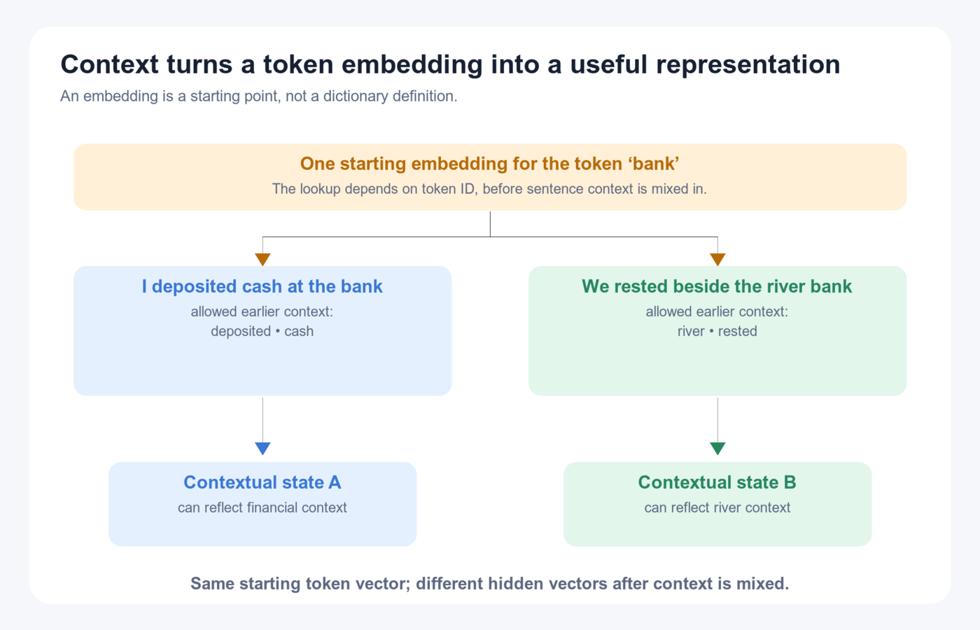
The picture follows one token position through this process. Its token ID and place in the sentence stay the same as the model's layers calculate new values for its hidden-state vector. The stored embedding row also stays unchanged during ordinary inference. What changes is the hidden-state vector carried forward for that occurrence. By the later stages, that vector can reflect the surrounding text as well as the original token.
Which surrounding words are allowed to contribute? In our left-to-right model, a position can use itself and earlier positions. At bank, both cash and river are earlier, so they are available in their respective sentences. At it in The animal stopped because it was tired, the words was tired are later. They cannot contribute to the calculation for it. This restriction also applies when training software processes a complete example at once: it must prevent later positions from leaking the answer into an earlier prediction.
The operation that lets one position combine information from other positions is called attention. The next sections show exactly what is multiplied and added. For now, remember the problem it solves: a token starts with an embedding vector selected by its ID, but useful predictions require hidden states that also depend on the available surrounding text. The input words themselves are not being rewritten.
Interview question: How do an embedding and a hidden state differ?
Reveal the answer after explaining it aloud
Answer: A token ID selects a stored embedding row. Two occurrences of bank with that ID start from the same row. As the model processes each sentence, earlier text contributes to new representation vectors, so the two occurrences can develop different hidden states. “Hidden state” names the vector at a particular stage; the initial embedding can be described as an initial hidden state, while later states include the effects of further calculations.
7. The problem attention solves
Return to The cat sat. For this example, treat each word as one token. The model now holds three representation vectors, each an ordered list of coordinates: one at The, one at cat, and one at sat. Our next task is to let information from the first two vectors affect the vector at sat. Later, the model will use that updated vector, after further calculations, to predict the next token.
Why is that necessary? Compare The cat sat with The committee sat. The last word is the same, but a suitable continuation may differ. If the calculation at sat used only the numbers for sat, it could not respond to this difference. Attention is the calculation that lets a position use numbers supplied by other allowed positions.
We will call sat the destination because that is where we need a result. We will call The, cat, and sat the sources because each can supply numbers for that result. The current position can be its own source. Keep this distinction throughout the calculation: these are positions already in the input, and the next output token has not yet been selected.
First understand what a weighted combination does
Suppose a teacher combines three test marks using a published rule: 20% from test one, 30% from test two, and 50% from test three. For marks 60, 80, and 90, the result is . The percentages tell us how strongly each mark contributes.
Those percentages are the weights in a weighted combination: a weight says how much to multiply a contribution by before adding it. Attention uses the same multiply-and-add idea. The model calculates the weights from the current input, so changing the input can change the weights. These attention weights are temporary calculation results; they are different from the stored model weights that training adjusts.
For sat, attention calculates three weights, one per source. Suppose a source supplies [2, 4] and receives weight 0.25. Its contribution becomes [0.25×2, 0.25×4] = [0.5, 1]. The model does this for all three sources, then adds their first coordinates to get the first result coordinate and their second coordinates to get the second. Section 9 calculates a complete example, including where the weights come from.
The result is another representation vector at sat, now influenced by earlier positions. Later calculations use that vector to score possible next tokens. Training adjusts the stored coefficients throughout this chain so that the final predictions improve; no step has to turn an intermediate vector into a human-readable sentence.
Why it is called self-attention
Here the destinations and sources belong to the same sequence, The cat sat. That is why the calculation is called self-attention. One version of the calculation—one set of rules for producing weights and combining source numbers—is an attention head. Section 12 explains why a model can run several heads for the same positions.
Every destination uses the input vectors that entered this layer. For example, calculating sat does not have to wait for this layer's new result at cat; it reads cat's input to the layer. The computer can therefore calculate these destination results together. For a model that predicts the next token, each destination may use itself and earlier positions. Section 11 shows how the program blocks later positions from contributing.
Interview question: What comes out of attention?
Reveal the answer after explaining it aloud
Answer: Each destination receives a list of numbers, or vector. The model makes it by multiplying each allowed source's numbers by that source's attention weight, then adding matching coordinates. Later model calculations still have to produce scores for possible next tokens and select a token.
8. Query, key, and value (Q/K/V)
For the sat position, attention needs to do two different things:
- Calculate how strongly each source should contribute.
- Obtain the numbers each source will contribute.
Queries and keys do the first job together. Values do the second.
Queries and keys are the two inputs to the scoring calculation
The model calculates a query from the representation at sat. It also calculates a key from each source representation: one for The, one for cat, and one for sat.
The model multiplies matching query and key coordinates, then adds the products. This is the dot product introduced earlier. It repeats the operation three times: sat's query with The's key, with cat's key, and with sat's key. The results are three scores. A later step turns those scores into the three attention weights that sum to 1; section 9 shows every calculation.
A score belongs to a pair: a destination and a source. “The score for cat” is incomplete unless we also say whose result we are calculating. When updating sat, we use the sat query. When updating cat, we use the cat query, and only the sources that position may read.
Values supply the numbers that the coefficients multiply
Each source also supplies a value, calculated from that source's representation. Once the temporary attention weights have been calculated, each weight multiplies the value from the same source. Add the results to obtain the attention output for sat. These multiplying coefficients are attention weights calculated for this input; they are not the stored model weights used to produce queries, keys, and values.
This is why key and value are separate. A key participates in calculating an attention weight; a value supplies the numbers multiplied by that attention weight. If we keep the query and keys unchanged but change the values, the attention weights stay the same while the final result can change.
| Object | Comes from | Used for |
|---|---|---|
Query for sat |
The representation at the destination sat. |
Scoring the allowed sources together with their keys. |
Key for cat |
The representation at the source cat. |
Calculating cat's score for the sat destination. |
Value for cat |
The same source representation at cat, through another transformation. |
Supplying the numbers multiplied by cat's calculated attention weight. |
Where do these three objects come from?
Recall what a matrix does: each output coordinate is a sum of input coordinates multiplied by stored coefficients. The model uses three such coefficient tables, called learned weight matrices, to turn each input vector into its query, key, and value. All positions use the same three projection matrices within this head. Training chose the matrix entries; answering a request uses those entries to calculate new vectors.
To write that calculation compactly, let mean the input vector at position . Let , , and be the three projection matrices. Multiplying the input by each matrix gives:
The subscript identifies a position, so means the query at position 3. Lowercase are one position's vectors. Put all input vectors in rows to form the input matrix ; put all resulting query vectors in rows to form . Then means “apply the query projection matrix to every input row.” The same convention gives and .
The query and key projection matrices contain different coefficients, so a position can be represented differently when receiving information and when supplying it. Even before applying a visibility restriction, sat's query compared with cat's key need not give the same score as cat's query compared with sat's key. The value projection matrix has a separate job: it produces the numbers to combine after the scores have determined the weights.
How does it learn which contributions are useful?
During training, the training program knows which token should follow the supplied text. It measures how poorly the model predicted that token, calculates how changes to the stored coefficients would affect the error, and adjusts the coefficients. That includes the query, key, and value projection matrices. There is usually no separate answer sheet saying which key a query must favor. A pattern such as using a sentence's subject can develop because it helps the final token prediction. Section 19 explains the error calculation and updates.
The names identify jobs performed by numbers. A query supplies the destination's input to scoring; a key supplies the source's input to scoring; a value supplies the source's contribution to the result. There is no English question or dictionary definition stored inside these vectors.
Analogy: preparing a report from several sources. Your information need helps you judge how useful each source is; the source's description helps with that judgment. These play the roles of query and key. The information you take from the source plays the role of value. A different report can give the same sources different importance. In the actual model, the comparison and contributions are numerical: the head combines weighted portions of several value vectors instead of retrieving one intact document.
The diagram is a map of the coming calculations. Section 9 explains “softmax”; section 11 explains scaling and masking. Read its plain-language labels first, then use the symbols to recognize the same steps in a formula.
Read diagram source
flowchart TB
    X["One input representation vector per position: X"]
    X -->|"Multiply by query projection matrix W_Q"| Q["Destination scoring vectors: Q"]
    X -->|"Multiply by key projection matrix W_K"| K["Source scoring vectors: K"]
    X -->|"Multiply by value projection matrix W_V"| V["Source contribution vectors: V"]
    Q --> C["Multiply and add query/key coordinates"]
    K --> C
    C --> D["Scale by square root of head width"]
    D --> M["Exclude sources this destination cannot read"]
    M --> A["Softmax: turn scores into attention weights totaling 1"]
    A --> S["Multiply source values by attention weights, then add"]
    V --> S
    S --> O["One output vector per query"]
Follow the two paths into the final combination. Queries and keys determine how much each source contributes. Values determine which numbers that source contributes. The program excludes forbidden sources before converting scores to attention weights. The examples use softmax without attention dropout. Changing only the values changes the supplied numbers while leaving those attention weights unchanged.
Interview answer: “For the position being updated, calculate a query. Compare it with each allowed source's key to obtain scores, then convert the scores into weights. Multiply each weight by that source's value vector and add. Query and key determine the weights; values supply the vectors being combined.”
9. Calculate one complete attention result
We will now calculate how the representation at “sat” can receive contributions from the three positions in “The cat sat”. We are still processing words already supplied to the model. We are not choosing the next word yet.
To keep every calculation visible, our example uses three input coordinates and just one number for each query, key, and value. A real head usually uses vectors with more coordinates. The method is the same.
Start with the inputs and the rules
These inputs are invented for the exercise:
| Position | Input representation | First coordinate | Second coordinate | Third coordinate |
|---|---|---|---|---|
| 1: The | [1, 0, 0] |
1 | 0 | 0 |
| 2: cat | [0, 1, 0] |
0 | 1 | 0 |
| 3: sat | [0, 0, 1] |
0 | 0 | 1 |
We also need rules that turn an input into its query, key, and value. In a trained model, training has learned these rules. Here we choose simple coefficients so you can check them by hand:
- Query rule: first coordinate + second coordinate + third coordinate.
- Key rule: 0 × first coordinate + 2 × second coordinate + 1 × third coordinate.
- Value rule: 2 × first coordinate + 10 × second coordinate + 4 × third coordinate.
Apply the same three rules to every row. For “cat,” for example, the key is 0×0 + 2×1 + 1×0 = 2, and the value is 2×0 + 10×1 + 4×0 = 10.
| Position | Query | Key | Value |
|---|---|---|---|
| The | 1 | 0 | 2 |
| cat | 1 | 2 | 10 |
| sat | 1 | 1 | 4 |
The number 10 does not mean that a cat is “ten units of meaning.” It is simply a computed intermediate number. Later learned calculations determine how such numbers affect predictions.
Step 1: calculate three scores for “sat”
We want an output at position 3. Therefore we use the query calculated at position 3: 1. Compare it with each available position's key. With one coordinate, a dot product is just multiplication:
| Contribution being considered | Calculation | Score |
|---|---|---|
| The → sat | sat's query × The's key = 1 × 0 | 0 |
| cat → sat | sat's query × cat's key = 1 × 2 | 2 |
| sat → sat | sat's query × sat's key = 1 × 1 | 1 |
All three positions are allowed because none is after “sat.” The normal attention scaling divides by the square root of the query/key width. Our width is 1, so we divide by 1; the scores remain 0, 2, 1. We will explain why wider heads need scaling in section 11.
Step 2: turn the scores into shares that add to 1
We need coefficients for combining the values. Scores can be negative and need not add to 1. Softmax converts them into positive attention weights, or shares: exponentiate each score, then divide by the total. The constant e is approximately 2.71828; raising it to a score makes larger scores receive larger positive numbers.
| Source position | Score | Exponential of score | Divide by total 11.107338 | Attention weight |
|---|---|---|---|---|
| The | 0 | e⁰ = 1 | 1 ÷ 11.107338 | 0.090031 |
| cat | 2 | e² ≈ 7.389056 | 7.389056 ÷ 11.107338 | 0.665241 |
| sat | 1 | e¹ ≈ 2.718282 | 2.718282 ÷ 11.107338 | 0.244728 |
The total is 1 + 7.389056 + 2.718282 ≈ 11.107338. The weights add to 1, apart from rounding. “cat” receives about 66.5% of the weight because its score was largest in this particular calculation. We did not assign that percentage separately.
Notice that a score of zero still gets some weight. Softmax turns zero into e⁰ = 1, not into zero.
Step 3: combine the values using those weights
The values are 2, 10, and 4. Multiply each by its attention weight and add:
This is the head's output at “sat.” It was calculated using contributions from all three positions, with the largest coefficient on “cat.” Real heads do the same calculation for every coordinate of their value vectors.
What does 7.81138 mean? By itself, it is neither a word nor a probability nor a fact. It is an intermediate result that subsequent model calculations use. The important change is that this result at “sat” now depends on earlier positions, including “cat.” Eventually, after many such operations, the model calculates scores for possible next tokens.
Use changes to the example to separate the three jobs
If we change “cat”'s value from 10 to 20 while holding queries and keys fixed, the attention weights stay exactly the same. The result increases by about 0.665241 × 10 = 6.65241. Values affect what is combined.
If we change “cat”'s key, its score can change, so the weights can change. If we change “sat”'s query, all three scores can change. Queries and keys affect how the combination is weighted.
Explain it back: “For the position I am updating, I compare its query with each allowed position's key. Softmax turns those scores into attention weights. I use those weights to combine the values. That produces a numerical attention output for the position—not the next token itself.”
Interview question: Does a 66.5% attention weight mean a 66.5% chance that ‘cat’ is the next word?
Reveal the answer after explaining it aloud
Answer: No. The 66.5% share multiplies the numbers supplied by the existing cat position in this attention head. After the remaining layers, a separate calculation will produce a score for each possible next token and turn those scores into token probabilities. That happens in section 18.
10. Extend the example from single numbers to vectors
A single number was enough to show the procedure. More coordinates let a head calculate richer combinations. We will now use two numbers per query, key, and value, while keeping the same three positions.
This is a second, fully specified teaching model. Its inputs and coefficients differ from section 9; its final answer therefore need not be the same. Nothing in these chosen numbers is a claim about the actual representations of “The,” “cat,” or “sat” in a production model.
Calculate Q, K, and V from the input
Each input now has four coordinates. Put one position on each row:
The first row is “The,” the second “cat,” and the third “sat.” Each of these particular rows has one 1 and otherwise zeros. This makes multiplication easy to inspect: each input selects the corresponding row of a projection matrix.
Here are the three projection matrices for this example. In a real model, they would contain coefficients learned during training; we choose their entries here so the calculation can be checked by hand. Each has four input rows and two output columns:
Read the first matrix as two query rules. Its first column combines the input coordinates using coefficients [1, 0, √2, 0]; its second uses [0, 1, 0, 0]. The square root of 2 is approximately 1.414. We deliberately chose it so that the scaling calculation below comes out neatly.
For “sat,” the input is [0, 0, 1, 0]. Its first query coordinate is 0×1 + 0×0 + 1×√2 + 0×0 = √2; its second is zero. Thus its query is [√2, 0]. Its key is [1, 1] and its value is [0, 4], obtained from the third rows of the other two matrices.
Multiplying all three input rows gives:
The capital letters collect all positions' vectors into matrices. Every row of Q, K, and V still refers to the same input position. A matrix's shape states its row count and column count. For example, means three position rows, each holding four coordinates. The equations below show that a matrix of three four-coordinate inputs, multiplied by a projection matrix with four input rows and two output columns, produces three two-coordinate outputs:
Calculate the output at “sat”
Use “sat”'s query with each key. In every line, multiply the first coordinates together and the second coordinates together, then add. For example, comparing [√2, 0] with [2, 0] gives √2×2 + 0×0 = 2√2:
Our query/key width is 2, so divide these scores by √2:
These are the same scores as in section 9's one-number example, so softmax gives the same weights: approximately [0.090031, 0.665241, 0.244728]. A single number is also called a scalar; the earlier example used scalars where this example uses two-coordinate vectors.
The values, however, now have two coordinates:
Combine the first coordinates to obtain the first output coordinate. Separately combine the second coordinates to obtain the second. Use the same attention weights for both:
The output at “sat” is therefore approximately [6.83247, 1.15898]. This is precisely what “a weighted sum of value vectors” means: repeat the multiply-and-add calculation coordinate by coordinate.
Calculate every position together
A model also needs outputs at the other positions. Matrix multiplication can calculate all query–key dot products in one operation. Transpose, written with a superscript T, exchanges rows and columns. Transposing K puts each position's key into a column, ready to be dotted with each query row:
The result has three rows for the three destination positions and three columns for the three source positions. Entry (3, 2) is the score for “cat” contributing to “sat.” It is not a score for the next word.
In full-sequence self-attention, queries and keys cover the same N positions, so the score matrix is square: N × N. Cross-attention can have different query and source lengths; incremental decoding can use one new query against many cached keys. Those score matrices need not be square.
Before converting scores to attention weights, the model must block sources a destination is not allowed to read; section 11 shows this masking step. It also applies the score scaling we used above. Then it applies softmax separately to each destination row. Call the resulting matrix of attention weights A. Each row has one weight per source, and its weights sum to 1 before any attention dropout. Multiplying A by V performs the weighted combination for every destination:
The Q and K widths must match to take dot products. The V width can differ: it determines the width of each head's output. For simplicity, our example made all three widths equal.
Interview question: Why is the attention score matrix square?
Reveal the answer after explaining it aloud
Answer: If all N positions supply queries and keys, every destination needs a comparison with every source: N rows and N columns. The dimensions change when the work changes. If we calculate only one new position's query against N stored keys, there is one row and N columns. If queries come from one sequence with Nq positions and keys from another with Nk positions, the score matrix is Nq × Nk. Section 17 calls that last case cross-attention.
11. Causal masking and scaled dot-product attention
We now know how attention combines positions. Two details make that calculation suitable for a next-token model: restrict which positions it can read, and control the scale of the scores.
Why the model cannot read later positions
Suppose a training example contains “The cat sat down.” We want the representation at “cat” to help predict “sat.” If that representation can already read “sat,” the model can copy the answer during training. It will not have that answer when asked to generate new text.
A causal mask prevents this shortcut. Position 1 may read position 1. Position 2 may read positions 1 and 2. Position 3 may read positions 1, 2, and 3. Reading the current position is allowed: at “cat,” the model is predicting the token after “cat.”
For our two-coordinate example, the scaled scores and mask together are:
Rows are destinations; columns are sources. The first row blocks columns 2 and 3. The second blocks column 3. The third can read all three.
The symbol −∞ means negative infinity. It is a mathematical way to make a forbidden position's softmax weight exactly zero, because its exponential is zero in the limiting calculation. Implementations use suitable masks or numerical representations; simply setting a blocked score to zero would be wrong, since e⁰ is 1.
| Query position ↓ / source key → | The (1) | cat (2) | sat (3) |
|---|---|---|---|
| The (1) | 0 · allowed | −∞ · blocked | −∞ · blocked |
| cat (2) | 0 · allowed | 0 · allowed | −∞ · blocked |
| sat (3) | 0 · allowed | 0 · allowed | 0 · allowed |
Read one row at a time. The bold diagonal is allowed: the representation at “cat” already knows “cat” and predicts the following token, “sat.” Adding mask value 0 leaves an allowed score unchanged; it does not give that position zero attention. A blocked score becomes −∞ before softmax, so its attention weight is zero.
A padding mask solves a different problem. A computer may process several examples together in a batch. To store them in a rectangular table, the program may extend shorter examples with dummy token positions called padding. Those dummy positions are storage placeholders, so the program excludes them as attention sources. A different mask may allow only a nearby window of positions. In each case, the mask states exactly which sources may contribute.
Implementation tip: boolean mask conventions differ between APIs. In PyTorch scaled-dot-product attention, True means allowed; in MultiheadAttention masks it means blocked. Set functional attention's dropout_p=0.0 explicitly for evaluation. For cached chunks, construct allowed sources from absolute token positions: a generic rectangular is_causal mask may align to the wrong corner. An entirely masked softmax row is undefined mathematically; follow and test the selected kernel's documented behavior. Padding-query outputs also need the appropriate loss/output mask. See the mask and cached-chunk examples and the PyTorch SDPA contract.
During training, the program has the complete example and can calculate all destination rows at the same time. The mask still limits each row to its prefix: the input from the start through that destination. Thus the row at cat can use The cat to predict sat, while the row at sat can use The cat sat to predict down. Both predictions can be calculated together without letting either read its answer.
Why divide a score by a square root?
A dot product adds one product per coordinate. Using more coordinates can make the sum vary over a wider range. What happens if two source scores become 0 and 10? Softmax gives approximately [0.000045, 0.999955]: almost the entire contribution comes from the second source. Scores of 0 and 1 instead give approximately [0.269, 0.731]. Dividing large scores by a suitable number helps prevent the head from making extremely one-sided combinations merely because its vectors are wider.
This also matters during training. The training program asks how a small change to a score changes the result; that rate of change is a derivative. When softmax is already almost entirely concentrated on one source, these derivatives can be very small. The score calculation then receives only a small signal about how to change. Scaling helps keep that part of learning responsive.
Why choose a square root for the divisor? We can estimate how much a dot product varies. The mean is the average. Variance measures spread by subtracting the mean from each value, squaring those differences, and averaging them. The standard deviation is the square root of that variance, so it describes spread in the values' original units.
For the estimate, assume the query and key coordinates vary independently, average to zero, and each have variance 1. “Independently” means knowing one coordinate does not tell us how another will vary. Under these assumptions, each query–key product has variance 1, and the variance of their sum grows with the number of products.
Here is the arithmetic for two independent products, each equally likely to be −1 or +1. Their four equally likely pairs give sums [-2, 0, 0, 2]. The average sum is 0, and its variance is (4+0+0+4)/4 = 2. After dividing every sum by √2, the squared values become [2, 0, 0, 2], whose average is 1. This illustrates the general rule: adding d independent products of variance 1 gives variance d and standard deviation √d. Dividing the sum by √d brings that standard deviation back to 1. Real learned coordinates need not follow the assumptions exactly; the estimate motivates the usual scaling.
For a width of 64:
Divide by 8, not by 64. In section 10, dividing by √2 turned [0, 2√2, √2] into [0, 2, 1]. In section 9, width 1 made the divisor 1.
What softmax does—and does not do
Write the allowed source scores as s₁ through sₙ, where n is the number of sources. The subscript j identifies the source whose share we want. In the denominator, r runs through all allowed sources and Σ means add their terms. Source j's attention weight, aⱼ, is:
The symbol Σ means “add up,” and r runs over the allowed sources in this destination row. Thus the denominator says “add every allowed source's exponential.” The numerator supplies just source j's exponential. Dividing by the common total makes the weights add to 1. A source's weight depends on its score relative to the other scores: raising a competing source's score can reduce this source's share even if its own score stays unchanged.
Very large exponentials can overflow a computer's number format. Subtracting the largest score from every score leaves softmax unchanged while avoiding unnecessarily large exponentials:
For example, subtracting 2 changes [0, 2, 1] into [-2, 0, -1]. Each new exponential is the corresponding old exponential divided by e². That divides both the numerator and the total denominator by the same number, leaving their ratio unchanged. The largest new score is zero, whose exponential is only 1, so unnecessarily large exponential values are avoided.
Ordinary softmax gives a positive mathematical weight to every source with a finite allowed score. A very small share therefore differs from the mask's exact exclusion. The largest share also does not, by itself, explain the model's final answer. It tells us how this head combined these values in this layer. Other heads, later calculations, and the direct additions explained in section 15 also affect the answer.
The familiar formula now describes operations we have done
Here is the whole calculation in one expression. Q collects the queries, K the keys, V the values, d_head is the number of query/key coordinates, and M is the matrix of mask additions. Softmax acts on one destination row at a time:
To evaluate it, start inside the parentheses: compare queries and keys → divide scores by √d_head → add the mask → turn each row's scores into attention weights → multiply those weights by V to combine source values. The last multiplication is why V is outside softmax.
Interview question: Why is a mask necessary when training targets are already known?
Reveal the answer after explaining it aloud
Answer: Targets are known to the training procedure so it can calculate errors. They must remain hidden from the model positions that are supposed to predict them. The mask enforces that separation.
12. Why a layer uses several attention heads
In section 10, sat used the attention weights [0.090031, 0.665241, 0.244728] for both output coordinates. One head must reuse its calculated attention weights across all its value coordinates. Suppose the model would benefit from one combination that favors cat and another that favors a different source. A second head lets it calculate that second combination at the same destination.
With several heads, the model produces several sets of attention weights and several resulting vectors. In the earlier backup-location question, one head might give more weight to a phrase naming the archive, while another uses a different combination of positions. Training can produce such behaviors by adjusting each head's projection matrices. The model designer chooses how many heads to provide, but does not assign a guaranteed “grammar” or “facts” job to each one.
In ordinary multi-head attention, each head has its own query, key, and value projection matrices. Each head performs the calculation we already worked through. The program then places the resulting output vectors side by side and multiplies this concatenated vector by another learned matrix, . This last multiplication is called the output projection. It turns all the heads' contributions into one vector with the width required by the next operation.
For example, head 1 might return [1, 2] and head 2 [3, 4]. Placing them side by side gives [1, 2, 3, 4]. If one output column of contains [1, 0, 1, 0], the corresponding output coordinate is 1×1 + 2×0 + 3×1 + 4×0 = 4. That coordinate uses contributions from both heads. Training learns the actual output coefficients.
In the formula, through are the H heads' outputs. Concat, short for concatenate, means place the output vectors side by side without changing their coordinates. For example, two four-coordinate outputs make eight coordinates. Multiplication by then combines those coordinates; merely joining the vectors does not perform that calculation.
Read the tensor dimensions as a description of the work
So far a matrix has organized numbers by row and column. With several sequences and heads, the program needs more labels to identify a number: which sequence, which head, which position, and which coordinate? An array organized along several such directions is called a tensor; each direction is an axis.
Suppose we process 2 sequences, each with 5 positions, using 2 heads, each with 4 query coordinates. The query array Q can have shape [2, 2, 5, 4]. Read it as “2 sequences; for each sequence, 2 heads; for each head, 5 query vectors; for each vector, 4 coordinates.” Each sequence/head pair makes a five-destination-by-five-source score matrix. The combined score array therefore has shape [2, 2, 5, 5].
Replace those counts by letters: B is the number of sequences in the batch, H the number of heads, N the number of positions, and d the coordinates per head. When Q, K, and V all use that width, their shapes are:
For each sequence and head, transposing K turns its N key rows of width d into d rows and N columns, so a query row can be compared with every key. The operation leaves the sequence and head labels alone. A software library may store these axes in a different order; check what each dimension means instead of identifying it only by its position in the shape.
A larger example has B = 2 sequences, N = 128 positions, model width 4096, and 32 query heads of width 128. The 4096 query coordinates per position are organized into 32×128 coordinates across the heads. Q has shape [2, 32, 128, 128]; its two final 128s happen to be equal but mean different things: positions and coordinates. Doubling the input length changes the first of those final two dimensions, not the head width.
Read diagram source
flowchart TB
    X["Input: one 8-coordinate vector per position"]
    X --> P["Calculate queries, keys and values for 2 heads"]
    P --> H1["Head 1: calculate attention weights and combine values"]
    P --> H2["Head 2: calculate attention weights and combine values"]
    H1 -->|"4 output coordinates"| C["Concatenate: 8 coordinates"]
    H2 -->|"4 output coordinates"| C
    C --> W["Multiply by W_O to combine head coordinates"]
    W --> Y["One 8-coordinate update per position"]
The heads form different weighted combinations in parallel. Concatenation places their output coordinates side by side; W_O then mixes those coordinates. These are learned pathways, not fixed human-assigned subjects.
Save cache memory by sharing keys and values
When the model generates a long answer, later tokens need to use earlier positions as attention sources. The program can save the earlier keys and values instead of recalculating them each time. This saved collection is the key/value cache, or K/V cache. It takes memory, and storing a separate set for every head increases that memory use. Section 22 follows cache use step by step; here we compare three ways to share the saved numbers:
| Design | Queries | Keys and values | With 32 query heads |
|---|---|---|---|
| Multi-head attention, MHA | Each head calculates its own queries | Each head calculates its own keys and values | Store 32 sets of keys and values per position |
| Grouped-query attention, GQA | Each query head calculates its own queries | A group of query heads uses the same keys and values | For example, store 8 sets; each is used by 4 query heads |
| Multi-query attention, MQA | Each query head calculates its own queries | All query heads use the same keys and values | Store 1 set, used by all 32 query heads |
Sharing keys does not force the attention weights to be identical: the query heads still have different queries. Sharing values does not make outputs identical either, because different weights can combine those shared values differently.
Think of several questioners consulting the same reference material. Sharing the material does not make their questions identical or force them to combine it in the same way. In GQA, the shared material corresponds to K/V and the different questions to Q. The calculation still uses learned vectors and weighted sums; there are no literal readers or documents inside a head.
MHA: four query heads read four K/V pairs.
Read diagram source
flowchart LR
    Q1["Q1"] --> K1["K1 / V1"]
    Q2["Q2"] --> K2["K2 / V2"]
    Q3["Q3"] --> K3["K3 / V3"]
    Q4["Q4"] --> K4["K4 / V4"]
GQA: four query heads read two shared K/V pairs.
Read diagram source
flowchart LR
    Q1["Q1"] --> K1["K1 / V1"]
    Q2["Q2"] --> K1
    Q3["Q3"] --> K2["K2 / V2"]
    Q4["Q4"] --> K2
MQA: all four query heads read one shared K/V pair.
Read diagram source
flowchart LR
    Q1["Q1"] --> K["K1 / V1"]
    Q2["Q2"] --> K
    Q3["Q3"] --> K
    Q4["Q4"] --> K
Each arrow means “this query head uses this set of keys and values.” The arrows show sharing, not a sequence of processing steps. In these four-query-head examples, MHA stores four sets per position per layer, GQA stores two, and MQA stores one. To compare their memory fairly, keep the same number of coordinates per key/value and the same numerical precision: the number format, and therefore the memory used to store each number.
Let count query heads and count the stored key/value sets, often called K/V heads. MHA stores sets; GQA stores . If the coordinate counts and storage format are unchanged, divide the latter count by the former to find the fraction of K/V memory retained:
With 8 K/V heads and 32 query heads, the fraction is 8÷32 = 1/4. With 8 and 64, it is 1/8. MQA with 32 query heads retains 1/32. These fractions describe the saved K/V numbers, not all model memory or total response time. Sharing changes what the heads can calculate, so a model designer must measure both answer quality and execution speed for the trained design.
Two shape details are useful in interviews. First, if each of H query heads produces d_v output coordinates, joining them gives H × d_v coordinates. then maps that concatenated vector to d_model coordinates, the model's usual width; those two widths need not already match. Second, when the program calculates just one new token per sequence and compares it with N source positions, the score shape is [B, Hq, 1, N]: batch, query head, one destination, N sources.
For the larger batched example above, 8 K/V heads give K and V shape [2, 8, 128, 128]. Each query head attends using its assigned K/V head. There are still 32 sets of query-head scores.
Interview question: Is an attention head an MoE expert?
Reveal the answer after explaining it aloud
Answer: An attention head combines contributions from different token positions. Mixture of Experts (MoE) names a different design: the model has several alternative networks for transforming one position's vector, and a learned selection calculation chooses which to use. Those alternatives are called experts and the selector is called a router. Section 14 explains the position-wise network; section 26 explains expert selection. A model can contain both attention heads and MoE experts.
13. Positional encodings: absolute, RoPE and ALiBi
Compare “Dog bites man” and “Man bites dog.” They contain the same words, but exchanging the first and last words changes who does the biting. The embedding lookup by itself gives a particular token the same initial embedding vector wherever it occurs. The model therefore needs another calculation that lets position affect the result.
Without position signals or an order-dependent mask, self-attention is permutation-equivariant: reordering the input positions reorders the output positions in the same way. The representations still depend on the tokens present, but their order does not change the relationships attention computes. Position mechanisms and causal masking change this setup.
The causal mask supplies one kind of order information: a position can read earlier positions and itself. It does not explicitly tell a query that a source is “three positions away” or that this is “position 17.” The following designs introduce position numbers or distances into the input vectors, query/key comparisons, or attention scores.
Option 1: add a position vector
Suppose the token representation is [0.2, 0.5] and the learned representation for position 3 is [0.1, −0.2]. Adding them gives [0.3, 0.3]. The same token at position 4 receives a different position vector, so its input to the next calculation differs.
Learned absolute position embeddings store one vector per supported position. “Absolute” means the vector refers to a location such as position 3, rather than directly to a distance between two positions. A position-embedding matrix trained for particular positions does not automatically work well at arbitrary unseen positions.
Instead of learning a position-embedding matrix, a program can calculate a position vector from a fixed rule. The original Transformer used sine and cosine for this. Picture a hand moving around a circle of radius 1: cosine gives its horizontal coordinate and sine its vertical coordinate. These coordinates repeat as the hand makes a full turn. Several hands moving at different speeds produce different combinations of readings as the position number advances.
That is the role of frequency here: how quickly a coordinate pair moves through its repeating pattern when the position number increases. The program calculates several such pairs, combines them into a position vector, and adds that vector to the token embedding.
The formulas measure angles in radians, rather than degrees. A full turn around the circle is 360 degrees or 2π radians, where π is approximately 3.14159; one radian is therefore about 57.3 degrees. In the notation, PE means positional encoding, pos is the token position, and d_model is the vector's number of coordinates. Counting coordinates from zero, pair i occupies coordinates 2i and 2i+1: i = 0 uses coordinates 0 and 1; i = 1 uses 2 and 3. The formulas are:
For a width of four, there are two pairs. Pair 0 divides pos by 10000⁰ = 1, so its angle is pos radians. Pair 1 divides pos by 10000^(2/4) = √10000 = 100, so its angle is pos/100 radians. The second pair advances around its circle 100 times more slowly. At position 1, the four-coordinate vector is approximately [sin(1), cos(1), sin(0.01), cos(0.01)] = [0.84147, 0.54030, 0.01000, 0.99995]. At position 2, it becomes approximately [0.90930, −0.41615, 0.02000, 0.99980]. The first pair changes substantially while the slower pair changes only slightly; together they supply a pattern tied to position.
At position 0, every pair instead starts at [0, 1]. The number 10,000 controls the pairs' rates, not the maximum allowed input length. Although the program can calculate a vector for a new position, the trained model must still be tested on inputs that long.
Option 2: rotate queries and keys before comparing them
There is another place to insert position information: change each query and key just before their dot product. Take two coordinates, view them as a point on a plane, and turn that point around the origin. The program chooses the angle using the token's position. Doing this to coordinate pairs throughout the query and key is called Rotary Position Embedding (RoPE).
A rotation changes direction while preserving the point's distance from the origin. For two coordinates written as a row vector, the calculation is:
Here θ is the rotation angle, and the primes in x′₁ and x′₂ mean “after rotation.” Multiplying out the matrix gives x′₁ = x₁ cos θ − x₂ sin θ and x′₂ = x₁ sin θ + x₂ cos θ. At θ = 90°, cosine is 0 and sine is 1, so [1, 0] becomes [0, 1]. At θ = 0°, it stays [1, 0]. In RoPE, each coordinate pair has its own rule for how far to rotate when the position number increases.
Why does this help? Rotating a query and a key by different angles changes their dot product. If both positions shift by the same amount, both receive the same extra rotation for this pair, which preserves that pair's dot product. The comparison can therefore depend on the difference between their positions. The worked example below makes this visible. Ordinary RoPE changes Q and K while leaving V alone, and each pair follows the model's chosen rotation rule rather than turning in 90° steps. The program still applies a causal mask afterward to exclude future sources.
When saving keys for reuse, programs commonly save the keys after rotating them for their positions. For example, a key computed at position 3 must retain position 3's rotation when a later query reads it. Applying its old rotation again, or treating a new token as position 0, changes the dot products and therefore the attention calculation.
To handle longer inputs, some designs change the rotation rates or map a larger range of positions into a smaller range before calculating angles; the latter is a form of interpolation. This extends the position calculation. It does not by itself show that the model can reliably use information near the end of a longer input, so the resulting model needs tests on those tasks.
Two positions make the relative effect visible
This calculation isolates the rotation before any causal mask. The final causal attention operation separately forbids a query from reading a future key.
Keep the unrotated content vectors fixed at q = k = [1, 0], and use a teaching frequency of 30° per position. At positions 1 and 3, their rotations are 30° and 90°. The vectors become [√3/2, 1/2] and [0, 1]; their dot product is 1/2. Shift both positions by one: positions 2 and 4 rotate by 60° and 120°, giving [1/2, √3/2] and [−1/2, √3/2]. The dot product is −1/4 + 3/4 = 1/2 again. The absolute positions changed, but their separation did not.
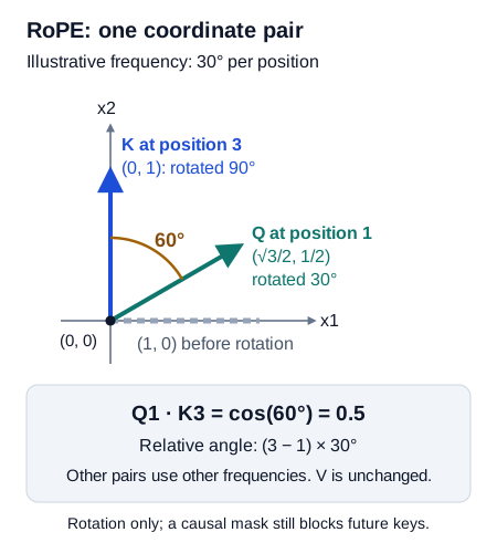
This invented example uses q = k = (1, 0) and a frequency of 30° per position. Position 1 rotates Q by 30°; position 3 rotates K by 90°. Their score depends on the 60° relative rotation. Real Q/K content differs and each coordinate pair has its own frequency; ordinary RoPE leaves V unchanged.
For ordinary fixed-frequency RoPE, adding the same rotation to both vectors preserves their dot product, so their relative rotation is what matters. A real head repeats this operation for many coordinate pairs at different frequencies. Programs usually express angles in radians, another angle unit in which a full turn is 2π rather than 360°. Also, the unrotated query and key depend on the surrounding text. We held those vectors fixed to isolate the position operation; moving a phrase in a real prompt may also change those input vectors. RoFormer describes the construction.
Option 3: adjust scores according to distance
A third approach leaves the vectors alone and adjusts the scores. The program calculates the distance between destination and source positions, multiplies it by a chosen positive number, and subtracts that amount from the source's score. A distant source therefore needs a stronger content score to receive the same share as a nearby source. This method is Attention with Linear Biases (ALiBi). “Linear” means the subtraction grows in direct proportion to distance:
Here i is the destination position and j the source position. The vertical bars in |i−j| mean take the nonnegative distance between them. The positive multiplier m, called the slope, determines the penalty per position of distance. The superscripts “content” and “adjusted” identify the score before and after subtraction. The causal mask still separately excludes future positions.
Suppose the destination is position 10, two earlier sources are at positions 9 and 4, and both content scores are 2. With m = 0.2, the adjusted scores are 2 − 0.2×1 = 1.8 and 2 − 0.2×6 = 0.8. The nearer source now has an advantage. Different heads use different slopes; sufficiently strong content can still outweigh the distance preference.
Compare the four position mechanisms
| Method | Where position enters | Learned position table? | What to remember about longer inputs |
|---|---|---|---|
| Learned absolute | Add the vector for a position to its input | Yes | Unseen positions require a supported adaptation; a fixed position-embedding matrix is not automatically unlimited. |
| Sinusoidal absolute | Add predetermined sine/cosine coordinates | No | Values can be computed outside training lengths; good behavior there is not guaranteed. |
| RoPE | Rotate query/key coordinate pairs | Not in the ordinary fixed-frequency construction | Preserve cache positions; frequency extensions must be validated with the trained model. |
| ALiBi | Subtract a distance penalty from scores, using the head's chosen multiplier | No position embedding table in the original scheme | The distance rule can handle larger numbers; test whether the model uses information beyond its training lengths. |
The table compares where the program inserts position information. The extra work differs: one method looks up and adds a vector, another rotates coordinates, and another modifies scores. The resulting time and memory cost depend on the software operations and hardware used. The original Transformer illustrates sinusoidal encoding, BERT illustrates learned absolute embeddings, and the documented Llama configurations in §31 illustrate RoPE. ALiBi's original paper describes how it was tested.
Interview question: Compare absolute embeddings, RoPE, and ALiBi.
Reveal the answer after explaining it aloud
Answer: Absolute embeddings add the embedding vector for a position to the token's input vector. RoPE rotates pairs of query/key coordinates using position-dependent angles, so their dot product can reflect the distance between positions. ALiBi subtracts a distance-based penalty directly from attention scores. All make position affect the calculation, but their ability to use much longer inputs must be tested with the trained model.
14. What happens after attention: transform each position's vector
Attention has brought numbers from other positions into the representation vector at sat. The next calculation works on that one vector: it forms new combinations of its coordinates, changes some of the resulting numbers, and produces an update of the original width. This gives later model calculations new numerical patterns to use when predicting a token.
This sequence of calculations is a feed-forward network (FFN). “Feed-forward” means the numbers move through these steps from input to output; this calculation has no loop that feeds its result back into itself. The program applies the same learned FFN weight matrices separately to every position. It does not fetch another position's vector during the FFN step. Earlier attention calculations have already put context into the input it receives.
A complete small example
Start with the vector [1, −2]. For this exercise, choose three rules for the first transformation: copy the first coordinate, copy the second, and add the two. The outputs are therefore [1, −2, 1+(−2)] = [1, −2, −1]. Two input coordinates have become three intermediate coordinates.
Next, keep each positive number and replace each negative number with zero; zero itself stays zero. Applying the rule separately to [1, −2, −1] gives [1, 0, 0]. This rule is named ReLU (Rectified Linear Unit).
Finally, calculate two output coordinates from the three intermediate ones. Let the first output be the first plus the third, and the second output be the second plus the third. From [1, 0, 0], this gives [1+0, 0+0] = [1, 0]. The result has the same two-coordinate width as the original input.
The complete path is [1, −2] → [1, −2, −1] → [1, 0, 0] → [1, 0]: expand, change numbers with ReLU, return to the starting width. We chose simple weight matrices to make the arithmetic visible. In a trained FFN, training adjusts the coefficients for the first and last transformations; the model designer chooses a rule such as ReLU for the middle step.
Why include the middle rule? A single multiplication rule cannot both keep positive numbers unchanged and set negative numbers to zero. Multiplying by 1 keeps both signs; multiplying by 0 removes both. ReLU changes its behavior depending on the input's sign. That makes it nonlinear. By contrast, two matrix multiplications in succession, with no such rule between them, can be combined into a single matrix multiplication. Adding more of those linear steps alone would not give this sign-dependent behavior.
A coordinate-changing rule such as ReLU is called an activation function. Its output is a calculated value—an activation—not a stored coefficient. Nonlinear activation functions let an FFN respond to input patterns in ways that one linear transformation cannot.
A common two-matrix FFN uses another coordinate-changing rule, GELU, which we calculate below. In this notation, x is one position's input row, and are its two weight matrices, and and are learned vectors added after multiplication. Those added vectors are biases. The intermediate result is h, and the final FFN update is y:
The first weight matrix produces d_ff coordinates, where d_ff names the FFN's intermediate width. The activation rule changes those numbers without changing their count. The second weight matrix returns to d_model coordinates, the usual model width. For model width 4 and intermediate width 12, follow the row and column counts:
The result must have the original width because the next step adds matching coordinates of this update and the existing vector. Section 15 shows that addition. Increasing d_ff increases how many numbers the FFN calculates at each position; it does not add token positions to the sequence.
GELU and SiLU: smooth alternatives to a hard cutoff
ReLU abruptly cuts off negative inputs. GELU (Gaussian Error Linear Unit) uses a smoother rule: multiply each input number by a fraction between 0 and 1 that becomes larger as the input increases. For example, an input of 1 receives a multiplier of about 0.8413, producing 0.8413. An input of −1 receives a multiplier of about 0.1587, producing −0.1587.
The exact multiplier is written Φ(z), pronounced “phi of z.” It is the fraction of area to the left of z under a bell-shaped probability curve with mean 0 and standard deviation 1, called the standard normal distribution. The definition can be written:
Here z is one input coordinate. The computer evaluates Φ(z) and multiplies it by z; the mathematical bell curve defines the multiplier and is not a claim that the model's coordinates must follow that distribution. Small negative inputs can therefore remain negative with reduced magnitude, rather than all being replaced by zero.
Another smooth rule is SiLU (Sigmoid Linear Unit), also called Swish in this form. It also multiplies an input by a fraction between 0 and 1, but calculates that fraction using a different formula. The multiplier is called sigmoid, written σ(z):
At z = 1, the sigmoid multiplier is 1/(1+e⁻¹) ≈ 0.7311, so SiLU returns 1×0.7311 = 0.7311. At z = −1, the multiplier is about 0.2689, so the output is about −0.2689. GELU and SiLU act on each coordinate separately. Unlike attention softmax, they do not compare a coordinate with all the others or force the output coordinates to sum to 1.
SwiGLU: let one computed branch modulate another
Instead of calculating only one expanded vector, an FFN can calculate two vectors from the same input using two different weight matrices. It applies SiLU to the first vector, then multiplies matching coordinates of the two vectors. For example, if the first vector after SiLU is [0.5, 2] and the second is [4, −3], their product is [0.5×4, 2×(−3)] = [2, −6]. A third weight matrix turns that product back into the model's usual width.
This design is SwiGLU, a Swish-based gated linear unit. Each separate calculation from the input is called a branch. The first branch is the gate because its numbers control how strongly the second branch's numbers pass into the product. Here is the same sequence in notation:
The input is x. and are the two expansion matrices; g and u are their resulting vectors after applying SiLU to the gate branch. The symbol ⊙ means multiply matching coordinates, producing h. is the third weight matrix, which turns h into the output update y.
The word “gate” means that one branch controls the size and sign of contributions from the other. A SiLU gate is not restricted to the range 0–1: it can be negative or greater than 1.
We can count the stored coefficients by counting weight-matrix entries. A basic FFN's expansion matrix has d_model × d_ff entries; its output matrix has d_ff × d_model. Together that is about 2 × d_model × d_ff parameters, ignoring biases. SwiGLU uses two expansion matrices and one output matrix, giving about 3 × d_model × d_ff. At the same intermediate width, 3÷2 = 1.5: 50% more parameters. Designers often choose a smaller gated intermediate width to keep the parameter count similar.
For a classic FFN with d_ff = 4 × d_model, the count becomes 2×d_model×(4×d_model) = 8×d_model². Ordinary MHA has four model-width matrices—query, key, value, and output—with about 4×d_model² entries together. Counting just these FFN and attention matrices, the FFN's fraction is 8/(8+4) = 2/3. Sharing keys/values with GQA, using a gated FFN, choosing several MoE experts, or changing the widths changes that count.
Interview question: What is the difference between attention and an FFN?
Reveal the answer after explaining it aloud
Answer: Attention brings together contributions from different allowed positions. The FFN works separately on each position's resulting vector: multiply by learned weight matrices, apply a nonlinear rule, and return an update of the original width. A usual Transformer block uses both, because combining positions and transforming their coordinates perform different jobs.
15. Residual connections, LayerNorm and RMSNorm
A model repeats attention and FFN calculations many times. How should one calculation's output become the next calculation's input? Two choices matter. First, we can add a proposed change to the current vector rather than replacing the vector outright. Second, we can rescale a vector before using it so that unusually large or small numbers do not dominate the following calculation. The first operation is a residual connection; the second is normalization. We will calculate both.
Residual connections: add an update to what is already there
Suppose the current vector is [1, 2, −1], and an attention or FFN calculation produces the update [0.2, −0.5, 0.1]. Add matching coordinates:
This is a residual connection:
Here x is the input vector, f is the attention or FFN calculation, f(x) is its proposed update, and y is the result after addition. The program keeps x available while calculating f(x), then adds matching coordinates. If f(x) were all zeros, y would equal x. A small update can therefore make a small adjustment without requiring f to recreate the original vector.
The addition also provides a direct mathematical path during training: changing a coordinate of x changes that same coordinate of the sum directly, as well as potentially changing f(x). This helps the training program calculate useful adjustment signals through many layers. It does not preserve a separate historical copy: an update of −1 added to a coordinate of 1 produces 0, so additions can cancel earlier information.
The vector carried through these repeated additions is called the residual stream. To add matching coordinates, the update and current vector must have the same width. That is why attention's output projection and the FFN's last weight matrix return to the model's usual width.
Think of a working draft receiving an edit: the edit can describe a change without restating the whole draft. That analogy explains why an update is useful. The actual model adds numbers and does not keep a recoverable document version for every layer.
LayerNorm: center and rescale one position's coordinates
Take the vector [1, 3]. We will first move its average to zero, then set a standard size for its spread. Calculate its mean: (1+3)/2 = 2. Subtract 2 from each coordinate to get [−1, 1]. Square those deviations and average them: ((−1)²+1²)/2 = 1, the variance. Divide both centered coordinates by the square root of 1, also 1. The result is [−1, 1].
This makes inputs with different overall offsets and scales easier for the next stored transformation to handle. For example, [10, 30] follows the same steps to become [−1, 1]: its mean is 20 and its standard deviation is 10. The model then applies learned multipliers and additions, allowing training to choose a useful scale and offset for each coordinate.
Layer normalization (LayerNorm) performs this kind of calculation across the coordinates of each position:
Read the symbols in the order of the calculation. μ (mu) is the coordinate mean, so x−μ subtracts that mean from every coordinate. σ² is the coordinate variance. ε (epsilon) is a small positive constant added before taking the square root, preventing division by zero when the coordinates have no spread. γ (gamma) contains one learned multiplier per coordinate; ⊙ applies those multipliers to matching coordinates. β (beta) contains one learned number to add per coordinate. The worked example omitted ε for easier arithmetic and used multipliers of 1 and additions of 0.
The program repeats this calculation separately for each position. It finds the mean and variance across that position's coordinates, not across different token positions. Its purpose is rescaling: the result may contain negative numbers and need not sum to 1. Softmax instead calculates positive shares that sum to 1.
RMSNorm: rescale without subtracting the mean
We can also control a vector's size without moving its mean to zero. For the same [1, 3], square the coordinates to get [1, 9], average them to get (1+9)/2 = 5, and take the square root: √5 ≈ 2.236. Divide the original coordinates by that value: [1/2.236, 3/2.236] ≈ [0.4472, 1.3416]. Unlike LayerNorm, this procedure kept both coordinates positive because it never subtracted their mean.
This is the core of root mean square normalization (RMSNorm):
In this formula, x² means square each coordinate and mean means average those squares. The square root of that average is the root mean square, which explains the name. The small positive ε again protects against division by zero. Finally, g supplies one learned multiplier per coordinate, applied with ⊙. Standard RMSNorm has these multipliers but no learned additive offset. It controls size while retaining a different result from LayerNorm, as [1, 3] showed.
Skipping mean subtraction removes operations from this calculation. Whether that noticeably speeds up the whole model depends on the hardware and implementation. Specialized hardware, such as a GPU (graphics processing unit), can perform many numerical operations together; hardware used to speed up a workload is called an accelerator. A kernel is a program that performs an operation on that device. A fused kernel combines several operations so that intermediate numbers need not be written out and read back between them. Such implementation choices, and the fraction of total time spent on normalization, affect the speed comparison.
Where normalization goes changes the block
Normalization can appear at different places in the repeated calculation. An attention operation or an FFN is often called a sublayer, meaning one major operation inside a full block. Write Norm for the chosen normalization calculation. In Post-LN, short for post-layer normalization, the program first calculates the sublayer's update, adds it to x, and then normalizes the sum:
In Pre-LN, short for pre-layer normalization, the program first normalizes a copy of x for the sublayer to use. It calculates the update from that normalized input, then adds the update to the original x:
For example, if x is [1, 3], a pre-normalized sublayer might receive the normalized [−1, 1], but its update is still added to [1, 3]. This distinction is the point of “pre.” The name Pre-LN is often used for this placement even when Norm is RMSNorm. Many decoder LLMs use pre-normalization inside blocks and an additional final normalization before producing vocabulary scores. The model's architecture specifies the actual placement.
Why placement changes the training path
To train the model, the training program calculates how changes to earlier numbers would change the final prediction error. It follows the calculation backward, a process called backpropagation. In Pre-LN, x reaches the output through direct addition as well as through the normalized sublayer. In Post-LN, the result of that addition must pass through normalization too. That extra operation changes the adjustment signals calculated during backpropagation. The difference helps explain why pre-normalization often makes a long stack of blocks easier to train.
The Pre-LN analysis by Xiong and colleagues examined these adjustment signals, called gradients, near the output layer when training first begins. It found large gradients for Post-LN in its analysis and more controlled gradients for Pre-LN. Large signals combined with large update steps can destabilize early training. Learning-rate warmup addresses this by starting with smaller update steps and gradually increasing them to the intended size. Pre-LN can help training, but designers still need to choose starting coefficients and update sizes carefully; they may still use warmup.
| Question | Alternatives | Independent choice? |
|---|---|---|
| What calculation normalizes the vector? | LayerNorm or RMSNorm | Yes: describes the operation. |
| Where is that operation placed? | Pre-normalization or post-normalization | Yes: describes the path through the block. |
Read diagram source
flowchart TB
    X["Current position vectors X"] --> N1["Normalize a copy of X"]
    N1 --> A["Attention: combine allowed sources in several heads"]
    A --> ADD1(("+"))
    X -->|"Keep original X for addition"| ADD1
    ADD1 --> H["H = original X plus attention update"]
    H --> N2["Normalize a copy of H"]
    N2 --> FF["FFN: transform each position separately"]
    FF --> ADD2(("+"))
    H -->|"Keep original H for addition"| ADD2
    ADD2 --> Y["Block output Y"]
Attention receives Norm(X), but its update is added to the original X. The FFN receives Norm(H), but its update is added to the original H. Both additions preserve the positions and model width. Each following block repeats this structure with its own learned parameters.
Interview question: Why do we need both residual connections and normalization?
Reveal the answer after explaining it aloud
Answer: A residual connection adds an attention or FFN update to the current vector, giving the current vector a direct path through the block. Normalization rescales a vector so the following calculation receives numbers with a more controlled size. Addition determines how an update joins the existing representation; normalization determines the numerical scale used in the calculation. A block can therefore need both.
16. Follow one whole Transformer block without losing the shapes
We can now follow the whole repeated calculation without changing the example midway. Start with 5 token positions, each represented by 8 numbers. Use 2 attention heads, each producing 4 coordinates, and an FFN that expands each position to 24 coordinates before returning to 8. The heads have separate query/key/value projection matrices, so this is ordinary multi-head attention (MHA). Normalize the input to each sublayer before calculating its update, as in the Pre-LN diagram above.
A block, often called a layer, is one complete group of these operations: attention, an FFN, normalization, and the additions that combine each update with the current vector. The output vectors of block 1 become the input vectors of block 2. The next block repeats the kinds of calculation but uses its own stored coefficients.
Read each row below as a change to those same five positions. A shape such as 5 × 8 means five position rows containing eight coordinates each. When a leading head dimension appears, 2 × 5 × 4 means two heads, each holding five position rows of four coordinates.
| Step | What it does | Shape after the step |
|---|---|---|
| Input | Hold one eight-coordinate representation for each of 5 positions | 5 × 8 |
| Normalize for attention | Rescale a copy of each position's coordinates; keep the original for addition | 5 × 8 |
| Project Q, K, V | Multiply by the query, key, and value projection matrices to get three sets of vectors | Each 5 × 8 |
| Split into heads | View each 8-coordinate vector as two groups of 4 | Each 2 × 5 × 4 |
| Compare queries with keys | Make a 5-by-5 score matrix for each head | 2 × 5 × 5 |
| Scale, mask, softmax | Divide scores by √4, exclude future sources, and calculate attention weights over sources for each destination | 2 × 5 × 5 |
| Combine values | Produce a four-coordinate output per position per head | 2 × 5 × 4 |
| Join heads; apply W_O | Put both head results side by side and combine their coordinates with the output projection matrix | 5 × 8 |
| Add original input | Add matching coordinates of the attention update and the saved original input | 5 × 8 |
| Normalize for FFN | Rescale a copy of the result; keep the original result for the next addition | 5 × 8 |
| FFN | At each position, expand to 24 coordinates, apply the activation rule, and return to 8 | 5 × 24 → 5 × 8 |
| Add FFN update | Add the update to the saved result of the first addition | 5 × 8 |
If this model uses rotary position embeddings, the program rotates the query/key pairs after calculating Q/K and before comparing them. If it uses a gated FFN such as SwiGLU, the FFN expansion produces two vectors of 24 coordinates per position. It multiplies the branch coordinates after applying the gate's activation rule, then uses the output projection matrix to produce eight-coordinate updates.
Several shape checks explain why the operations fit together. Normalization keeps the number of positions and coordinates:
For each head, comparing five four-coordinate queries with five four-coordinate keys gives:
There are two such score matrices, one per head. The five rows are destinations, and the five columns are sources. Multiplying a 5 × 5 attention-weight matrix by 5 × 4 values returns 5 × 4 outputs. Joining the two head outputs gives 5 × 8.
The final block operation has compatible shapes because the FFN returns to width 8:
The block began with five positions and ends with five updated positions. It has changed their numbers, not added new tokens. The model passes those results through the remaining blocks. Only after the last block does it apply any configured final normalization and the vocabulary projection matrix that produces one score per candidate token; section 18 explains that last matrix.
If the vocabulary contains 100 entries, the last position's eight-coordinate vector becomes 100 scores:
During training, the program knows the next token after each input position, so it can apply this vocabulary projection matrix wherever it has a target to check. Such a position is called supervised because its correct next token is supplied. During ordinary generation, the model needs the scores from the last prompt position to choose the first new token. It does not generate five new tokens merely because this block processed five input positions.
How this chapter connects to the next three
This chapter explains the complete path from text to model behavior. Use the following chapters for deeper treatment after that path makes sense:
- Tokenization Deep Dive: how text becomes IDs, including vocabulary construction and practical tokenization effects.
- Attention Mechanisms: variants of the score-and-combine operation, its shapes, and its costs.
- Transformer Architecture: how blocks, normalization, positions, and architectural choices fit together.
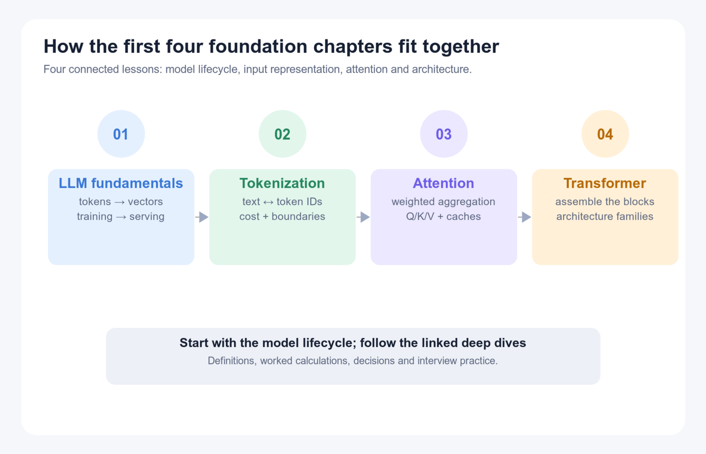
Interview question: Why doesn't a 32-layer model have 32 times as many token positions at the end?
Reveal the answer after explaining it aloud
Answer: Thirty-two layers means the model transforms the position vectors 32 times. Each block still returns one vector of the usual width for each position it received. The sequence grows when the program selects and appends a new token, not when the current vectors pass through another block.
17. Which kind of Transformer are we describing?
So far, each position has read itself and earlier positions to help predict the following token. A model built from blocks that operate this way is called a decoder-only Transformer. This design directly supports writing a continuation one token at a time. Other Transformer designs use similar numerical operations but change which positions can read one another and what output the model is trained to produce.
| Family | What can read what? | Typical output and use | Public example |
|---|---|---|---|
| Encoder-only | Each supplied input position can usually read earlier and later supplied positions | Produce input vectors used to label text, locate an answer inside text, or compare text with search candidates | BERT |
| Decoder-only | Each position reads itself and earlier permitted positions | Select the next token, append it, and repeat; this is called autoregressive generation | Llama |
| Encoder–decoder | One network represents the whole source; another reads those source vectors plus its own permitted output prefix | Generate text from a separate supplied source, such as translating a complete sentence | T5 |
Bidirectional means a position can read both directions within the supplied input. For example, to fill the blank in The ___ sat, a model can use both The and sat. In BERT-style masked-language training, the training program hides or alters selected tokens and asks the model to predict their original identities from the available surrounding text. That differs from our next-token task, where The cat must predict sat without reading it. An encoder's access to both directions concerns supplied text, not text the user has yet to provide.
Cross-attention uses one sequence to read another
Suppose the input is a complete English sentence and the desired output is a French translation. The encoder first produces a vector for each English input position, using the supplied source sentence. As the decoder generates French text, it needs to consult those English vectors. It calculates queries from its French-side representations and keys and values from the encoder's English-side outputs. This use of two different sequences is cross-attention.
The model still compares each query with keys, turns the scores into attention weights, and combines values. If it has Nq decoder query positions and Nk encoded source positions, it needs Nq rows of Nk comparisons:
For example, two decoder positions consulting five source positions give a 2 × 5 score matrix. The decoder separately uses causal self-attention over the French tokens supplied or generated so far. “Self” therefore means queries, keys, and values come from the same sequence; “cross” means the queries come from one sequence and keys/values from another. Both use the attention calculation we already learned.
Choose the family from the task
Start by stating the output the application needs. If it needs a label such as refund request, it can calculate a vector for the supplied message and use that vector to score possible labels. If it needs an extracted span, meaning a stretch of the supplied text, it can score which input positions start and end that span. Encoders support these uses. A causal decoder directly supports writing new text one token at a time. An encoder–decoder provides a separate representation of the complete source while writing the output. Decoder-only models can also label or translate text when prompted or trained for those tasks, so architecture suggests candidates rather than deciding the result by itself.
| Task | Candidate starting point | What to measure before choosing |
|---|---|---|
| Label millions of short support messages | An encoder trained for the task plus a classification head, a final calculation that scores the labels | Correct-label rate; whether confidence agrees with actual correctness (calibration); messages processed per second; model memory; and retraining cost. |
| Generate open-ended responses | A causal decoder trained on examples of following instructions | Useful answer quality; how much input it can use; time to produce an answer; and behavior on requests it should handle carefully. |
| Translate or summarize a distinct source | An encoder–decoder or a decoder-only model suited to the task | Preservation of source meaning; output quality; available training examples; and total execution cost. |
Try the decision: a product needs one of eight labels describing why a customer contacted support. Compare a compact model trained to choose those labels with a text-generating model prompted to return a label. Measure errors, confidence, processing rate, and cost on representative messages. Choose the classifier if those measurements meet the product's needs. The name “encoder” alone does not establish that a particular model is smaller or faster.
Why Transformers mattered
An earlier recurrent neural network (RNN) carried a vector—an ordered list of numbers—called its state, from one token to the next. To calculate the state for token 3, it first needed the newly calculated state for token 2. A long short-term memory network (LSTM) is a recurrent design with learned gates that control how much of its stored information to retain, replace, and expose. Those gates help manage information over a sequence, but the next state still depends on the preceding state. That forces work along the sequence to happen in order.
An attention layer instead receives all the input vectors for that layer at once. The output at position 3 can consult the input vector at position 1 directly, without waiting for the layer's new output at position 2. When the sequence is known, the computer can calculate many destination rows together. This helps train large models using hardware that performs many calculations at once. The cost is the number of comparisons: ordinary dense attention calculates a full destination-by-source score matrix. Doubling the length from N to 2N changes its size from N × N to (2N) × (2N)—four times as many entries.
During ordinary autoregressive generation, the next input token has not yet been chosen. The program must select it before calculating the step that uses it. Thus a Transformer can process known positions together during training while still generating a new continuation one token at a time.
A recurrent layer: each new state needs the preceding state.
Read diagram source
flowchart LR
    R1["Use token 1 to calculate state 1"] --> R2["Use token 2 and new state 1 to calculate state 2"]
    R2 --> R3["Use token 3 and new state 2 to calculate state 3"]
A causal attention layer: all query rows can be calculated together.
Read diagram source
flowchart TB
    X["All known position vectors entering this layer"]
    X --> A["Query 1 reads source 1"]
    X --> B["Query 2 reads sources 1 and 2"]
    X --> C["Query 3 reads sources 1, 2, and 3"]
    A --> O["Three updated position vectors"]
    B --> O
    C --> O
The Transformer rows depend on the states entering the layer, not on another row's just-computed output in that same layer. The causal mask still excludes later source positions. This parallelism applies when the sequence is known; stacked layers and newly generated tokens still have dependencies.
Interview question: Can an encoder-only model serve as a chatbot in exactly the same way as a causal decoder?
Reveal the answer after explaining it aloud
Answer: A usual encoder produces vectors for supplied input and is trained for tasks such as predicting hidden input tokens. That alone does not supply the same “predict the next token, append it, repeat” procedure as a causal decoder. An application can still use an encoder to find relevant text or interpret an input, then pass its result to a generator. To decide what a system can do, inspect the model's allowed information flow, training task, and the application around it.
18. Turn the final representation into an actual token
The last block has returned a hidden-state vector for each supplied position. To continue The cat, the program uses the final hidden state at cat to score possible next tokens. The candidates come from the tokenizer's vocabulary: the complete list of token IDs the model can select. We will first calculate candidate scores, then turn those scores into probabilities, then choose one ID.
Each candidate has a column of stored coefficients. The program multiplies matching entries of the final position's vector and that candidate's column, then adds the products. For example, vector [2, 1] and candidate column [0.5, −1] give score 2×0.5 + 1×(−1) = 0. A different candidate column [1, 0] gives score 2. Applying all candidate columns together is a matrix multiplication called the language-model head, or vocabulary projection.
With a representation width of 4 and a vocabulary of 10,000, the vocabulary projection matrix has four input rows and 10,000 output columns. One position therefore produces 10,000 scores:
In the formula, h is the final position's vector and is the vocabulary projection matrix. The resulting raw scores are called logits. Because they are multiply-and-add results, logits can be negative or larger than 1; they do not yet say how often a token should be selected.
The program applies softmax to these candidate scores: exponentiate each, then divide by the total. That gives one positive probability per candidate, with the probabilities adding to 1. This vector of probabilities is the next-token probability distribution. Softmax performs the same arithmetic as it did in attention, but answers a different question. Here the probabilities describe candidate vocabulary entries. In attention the weights described source positions contributing values.
The input embedding table already holds a vector for every vocabulary entry. Some models reuse those stored numbers when scoring outputs: turn each embedding row into a candidate column by transposing the table. Its shape changes from vocabulary × model-width to model-width × vocabulary, exactly the shape needed above. This sharing is called weight tying. It saves the memory needed for a separate output projection matrix. Other models learn separate input embedding and output projection matrices.
Decide how to select from the distribution
Suppose the next-token probabilities are [0.50, 0.30, 0.15, 0.05]. One selection rule simply chooses the first candidate because 0.50 is largest. Repeat that rule after every new token: this is greedy decoding. “Greedy” describes taking the highest-probability choice at the current step. Because that choice changes the next step's probabilities, it need not produce the most likely complete sequence—or the most useful answer.
Optional depth: a branching example and beam search
Suppose two first tokens have probabilities A = 0.6 and B = 0.4. After choosing A, the most likely second token has probability 0.5. After choosing B, the most likely second token has probability 0.9. Multiply the probability of the first choice by the probability of the second choice given that first choice to score a two-token path. Greedy chooses A and gets 0.6 × 0.5 = 0.30; the best path beginning with B gets 0.4 × 0.9 = 0.36. This example ends after exactly two choices. At each branch, other possible second tokens account for the remaining probability.
Instead of retaining only the best next choice, beam search retains a chosen number of promising unfinished sequences. That number is its beam width. A width-two beam can keep both A and B in this example, extend both by candidate second tokens, and compare the completed paths. With a larger tree of possibilities, even a beam can discard a path that would have become best later.
Programs usually store a sum of log probabilities instead of multiplying many small probabilities. A logarithm undoes exponentiation: the natural logarithm ln(p) asks “what power of e gives p?” The identity ln(a×b) = ln(a)+ln(b) lets the program add these scores while ranking fixed-length sequences in the same order as their probability products. Programs may also adjust scores for sequence length and set rules for when to stop. Finding a high-probability sequence according to the model still does not prove it true or useful. Beam search searches among partial sequences; the sampling controls below instead modify the probabilities used to draw a next token.
Another rule makes a random choice using the probabilities. Imagine 100 tickets: 50 name the first candidate, 30 the second, 15 the third, and 5 the fourth. Drawing one ticket implements the example distribution. This is sampling. The second candidate can be chosen even though its 0.30 probability is not the largest. Repeating the same draw many times would select it about 30% of the time. In a model, selecting it then changes the input for the next step. Sampling creates variation, which can help produce different candidate answers but can also choose less suitable tokens.
Before sampling, the program can increase or decrease the gap between candidate logits. Divide every logit by a chosen positive number T, then apply softmax. This setting is called temperature. A divisor below 1 makes the score differences larger; a divisor above 1 makes them smaller:
Here zᵢ is candidate i's original logit and zᵢ⁽ᵀ⁾ its adjusted logit. For [2, 1], compare the adjusted scores and their softmax probabilities:
| Temperature | Scaled logits | Probabilities |
|---|---|---|
| 0.5 | [4, 2] |
About [0.881, 0.119] |
| 1 | [2, 1] |
About [0.731, 0.269] |
| 2 | [1, 0.5] |
About [0.622, 0.378] |
A lower positive temperature gives the already favored candidate more probability; a higher one moves the candidate probabilities closer together. An API—a software interface through which an application requests a model result—may accept “temperature 0” as a special greedy or near-greedy setting. The implementation cannot literally divide by zero. Reducing temperature also cannot repair an incorrect high-scoring answer, and execution details can still prevent exactly repeated outputs.
The program can also remove low-ranked candidates before drawing. Top-k keeps a fixed number k of the highest-probability candidates. With [0.50, 0.30, 0.15, 0.05] and k = 2, only the first two remain. Their old probabilities add to 0.80. Divide each by 0.80 to make the remaining candidate probabilities add to 1: [0.50/0.80, 0.30/0.80] = [0.625, 0.375]. This rescaling is called renormalization. The removed candidates have zero chance in that draw.
Top-p, also called nucleus sampling, chooses how many candidates to retain by their total probability. Sort the candidates from highest probability to lowest, then include them until their running total reaches the chosen threshold p. With the same distribution and p = 0.90, the first two total 0.80, so include the third to reach 0.95. Divide the retained probabilities by 0.95 before sampling. If a different distribution's first candidate already had probability 0.95, that one candidate would meet the threshold. Top-p therefore retains a variable count of candidates; top-k retains a chosen count.
These controls can be combined, but order matters: temperature can change the probabilities that a top-p filter sees. Programs may also lower scores for candidates such as recently repeated tokens. To predict the behavior of a particular service, check which operations it applies and in what order.
Continue until a stopping condition is met
After selecting an ID, the program appends it to the sequence and uses the extended input to calculate the following token's probabilities. It repeats until a stopping rule applies. A model may select a special end-of-sequence token, whose role is to signal completion. Alternatively, the application may stop after a chosen token limit or when the output matches a configured stop sequence, such as a particular string or sequence of token IDs.
To display the answer, the tokenizer converts the generated IDs back into their text or byte pieces and joins them. A displayed word may need several generated tokens. Some model outputs instead use special control tokens or a structured description of a tool call. The application reads that structure and decides which action to perform; selecting its token IDs does not itself execute a tool.
Interview question: Does temperature control creativity?
Reveal the answer after explaining it aloud
Answer: Temperature divides the token scores before softmax. Lower positive values make sampling more strongly favor the already highest-scoring candidates; higher values spread probability more widely. This changes variation in the selections. Whether the result is usefully creative still depends on what the model knows, the request, and how candidate answers are judged. It does not directly set correctness or intelligence.
One complete tiny decoder: IDs all the way to a selected token
We have calculated the model components separately. Now follow one unchanged set of inputs and weight matrices all the way from token IDs to a selected next token. The program looks up the IDs, adds position vectors, runs a complete decoder block, and calculates vocabulary probabilities. It then chooses a token and processes that choice to choose another token. We will also compare saving earlier keys/values with recalculating the whole input, to check that saving them preserves the result.
Download the runnable tiny decoder. This Python program contains all the weight matrices and the arithmetic used below. Python's included libraries are sufficient to run it; there is no trained model to download. You can follow the table without knowing Python, then use the program to inspect or change the numbers.
This is a new teaching model, not the same set of coefficients as the isolated attention examples. We chose its numbers to make the full calculation small enough to inspect. The model has one block, one attention head, two coordinates per position and per head, an FFN that expands to three coordinates, and only four vocabulary entries. The recognizable token names help us track the calculation; the chosen numbers have not learned English. Its complete embedding table is:
| Token | ID | Embedding row |
|---|---|---|
The |
0 | [1.0, 0.0] |
cat |
1 | [0.0, 1.0] |
sat |
2 | [1.0, 0.2] |
. |
3 | [-1.0, 0.0] |
Its tokenizer splits text wherever there is a space, so write punctuation separately: The cat sat .. It does not use byte-pair encoding (BPE). Positions are counted from zero: the first token is at position 0, the second at position 1, and so on. The model has four absolute position vectors, [0, 0], [0.1, −0.1], [0.2, −0.2], and [0.3, −0.3], for positions 0 through 3. It has no vector for a fifth token at position 4.
Three operations use RMSNorm: before attention, before the FFN, and before vocabulary scoring. Each uses ε = 0.000001 inside the denominator and multipliers [1, 1] afterward. These fixed multipliers stand in for the scale parameters that a real model could learn. The FFN uses ReLU, and the projection matrices have no separate bias vectors to add.
Start with The cat. The tokenizer returns IDs [0, 1]. The last token, cat, has ID 1, which selects embedding row [0, 1]. It is the second token, at position 1, so add [0.1, −0.1]: [0+0.1, 1−0.1] = [0.1, 0.9]. Follow this vector through the block in the table below. The program also processes the preceding The position because attention at cat needs the numbers it supplies.
The following pseudocode states the operations in execution order. It is a reading guide, not Python you must understand before continuing. Each variable on the left stores the result calculated on the right. The last line chooses an ID; it does not yet process that chosen token through the block.
X = embedding_lookup(token_IDs) + absolute_position_vectors
A = RMSNorm(X)
Q, K, V = A @ W_Q, A @ W_K, A @ W_V
scores = Q @ transpose(K) / sqrt(2)
scores[future_source_positions] = negative_infinity
weights = softmax(scores, over_source_positions)
attention_update = (weights @ V) @ W_O
H = X + attention_update                         # first residual
expanded = RMSNorm(H) @ W_UP                     # width 2 -> 3
ffn_update = ReLU(expanded) @ W_DOWN              # width 3 -> 2
Y = H + ffn_update                               # second residual
final = RMSNorm(Y)
logits = final @ W_LM                            # width 2 -> vocabulary 4
probabilities = softmax(logits, over_vocabulary)
selected_ID = argmax(probabilities[last_position])
Here @ means matrix multiplication, transpose exchanges rows and columns, and sqrt(2) is the square root of the head width. W_UP and W_DOWN are the FFN expansion and output matrices; W_LM is the vocabulary projection matrix. argmax returns the position of the largest entry, which here is the selected vocabulary ID. last_position tells the program to use the final prompt position's probabilities for that choice.
The actual Python program enforces the same causal mask by supplying each destination only itself and earlier sources. No future source enters its softmax. There is just one attention head, so no output vectors from separate heads need to be joined, but W_O is still present to transform that head's result before addition.
The table follows cat. Read down the middle column to see the changing activation vector; use the last column to check what it is for at that point. Values are rounded to six decimal places for display. The program uses the computer's floating-point number format, which keeps more digits but still represents most real numbers approximately.
| Operation | Result at cat |
What that result means |
|---|---|---|
| Embedding + position | [0.100000, 0.900000] |
The block's input at position 1 |
| Attention RMSNorm | [0.156174, 1.405562] |
Rescaled copy used to calculate queries, keys, and values |
| Query projection | [0.078087, 0.702781] |
The query used to score both allowed sources |
| Key projection | [-0.265495, 1.436797] |
This position's source key |
| Value projection | [0.156174, 0.702781] |
This position's contributed coordinates |
Scaled scores over The, cat |
[0.218643, 0.699344] |
Two query–key comparison scores |
| Attention softmax | [0.382087, 0.617913] |
Attention weights over the two source positions |
| Weighted sum of values | [0.636853, 0.434258] |
The head's output |
| W_O projection | [0.405278, 0.280814] |
Head output multiplied by the output projection matrix; the update to add |
| First residual | [0.505278, 1.180814] |
Input plus attention update |
| FFN RMSNorm | [0.556355, 1.300179] |
Rescaled copy of the first addition's result, for the FFN |
| W_UP projection | [1.206445, 0.743824, −0.371912] |
Three intermediate coordinates |
| ReLU | [1.206445, 0.743824, 0.000000] |
The negative coordinate has been set to zero |
| W_DOWN projection | [0.241289, 0.148765] |
The two-coordinate FFN update |
| Second residual | [0.746567, 1.329579] |
First residual plus FFN update: the block output |
| Final RMSNorm | [0.692403, 1.233117] |
The final vector used to score candidate tokens |
| Vocabulary projection | [-0.962760, 0.261792, 1.233117, 0.692403] |
Logits for The, cat, sat, . in ID order |
| Vocabulary softmax | [0.053693, 0.182698, 0.482585, 0.281025] |
Probabilities over the four vocabulary entries |
For example, the preceding The position supplies value [1.414212, 0]. Multiply it by its share 0.382087 and multiply cat's value [0.156174, 0.702781] by its share 0.617913. Adding matching coordinates gives approximately [0.636853, 0.434258], the head's output. W_O transforms that output to [0.405278, 0.280814]. Adding it to the original [0.1, 0.9] gives [0.505278, 1.180814], the first residual result. Each row is therefore a different stage of one calculation, not a separate illustrative number.
Notice the two different normalized distributions. Attention gives the larger attention weight to the existing cat position. The later vocabulary softmax gives its largest candidate probability to sat. The first determines which existing numbers contribute; the second helps choose which token to append.
At the bottom of the table, the language-model head's column for candidate sat is [0, 1]. Its logit is therefore 0.692403×0 + 1.233117×1 = 1.233117. Softmax compares this score with the other three candidate scores. Greedy selection chooses ID 2, sat, because its probability, approximately 0.482585, is largest. A probability below 0.5 can still be the largest when there are several candidates.
Now process the chosen token. After processing the prompt, the program saved keys and values for The and cat, so the cache contains two positions. Selecting ID 2 added sat to the displayed sequence, but has not yet calculated a key or value for it. To choose the following token, embed sat at position 2: [1.0, 0.2] + [0.2, −0.2] = [1.2, 0]. Calculate its query, key, and value; save its new key and value beside the older ones; and complete attention, the FFN, and vocabulary scoring for this position. The next probabilities are [0.067904, 0.191047, 0.154313, 0.586736], so the next chosen ID is 3, ..
To check the shortcut, the program independently processes the entire known prefix [The, cat, sat] again from its IDs. It compares those results with processing only the new token while reusing the saved keys/values. It requires the numerical differences to stay below 10⁻¹², or 0.000000000001; that allowed difference is the test's tolerance.
The cache now holds three processed positions, while the display contains four tokens: The cat sat .. The final period has been chosen but not processed. We deliberately stop after two generated tokens. Here . is an ordinary vocabulary entry, not a special instruction to stop. Because the demonstration ends, the program has no reason to run another forward pass, meaning another calculation from that token's input through the model to output scores.
A small bridge back to training. We chose a token using fixed weight matrices. Now suppose a training example supplies the answer: sat should follow The cat. The program can measure its prediction error and adjust some stored coefficients. To keep this check small, the script makes a copy of the vocabulary projection only and keeps the final input vector fixed.
The error measure, or loss, is called cross-entropy. For one correct next token, it is −ln(probability assigned to that token). The natural logarithm ln(p) asks what power of e, approximately 2.71828, gives p. For probabilities below 1 that power is negative, and the minus sign makes the loss positive; probability 1 gives zero loss. For sat, −ln(0.482585) is approximately 0.728599. Section 19 develops why lower correct-token probability produces a larger penalty.
For this softmax-and-loss combination, the derivative of the loss with respect to one candidate's logit is predicted probability − target indicator. The target indicator is 1 for the correct token and 0 for the others. For sat, that gives approximately 0.482585−1 = −0.517415: raising its score would reduce this example's error.
Now follow one stored coefficient. The sat scoring column is [0, 1], and the final input vector is [0.692403, 1.233117]. If we increase the column's second coefficient by δ, read “delta,” meaning a small change, the sat logit increases by 1.233117×δ. Near the current values, each small logit increase changes loss at the rate −0.517415. Combining the two effects, the loss changes by approximately −0.517415×1.233117×δ = −0.638033×δ. The coefficient's loss derivative is therefore about −0.638033. Following how one change affects the next calculation this way is the chain rule, developed further in section 19.
With learning rate 0.1, update this coefficient by subtracting the learning rate times its derivative: 1 − 0.1×(−0.638033) ≈ 1.063803. The stored coefficient increases, which raises the correct token's score for this fixed input vector. The program calculates a corresponding derivative and update for every coefficient in the copied vocabulary projection matrix.
The script uses these derivatives to update all coefficients in the copied vocabulary projection matrix: subtract learning rate × derivative from each. With a learning rate of 0.1, this one update lowers the example's loss from 0.728599 to 0.654798. The script has changed actual stored coefficients, but only in the copied vocabulary projection matrix. Training the whole model would also follow the calculation backward through the blocks and embeddings to update their parameters. The weight matrices used to generate the example remain unchanged because this training check updates a separate copy.
After downloading the file, run:
python3 01-llm-internals-tiny-decoder.py
From a checkout of this repository, run:
python3 override/01-foundations/examples/01-llm-internals-tiny-decoder.py
The program prints every vector in the table and finishes with the following checks. Prefill means the initial processing of all known prompt tokens; “cached next step” means processing the selected next token while reusing the earlier saved keys and values. Section 22 explains the performance consequences of those two phases.
Greedy token after prefill: sat (ID 2)
Full-prefix and cached next step agree (tolerance 1e-12).
Next-step probabilities: [0.067904, 0.191047, 0.154313, 0.586736]
Next greedy token: . (ID 3)
Displayed tokens: The cat sat .
Cache contains 3 processed positions; the last selected token is not processed.
Head-only training on target 'sat': loss 0.728599 -> 0.654798.
Only a copy of W_LM was updated; this is not full-model backpropagation.
Predict before changing it: If the last token of a known sequence changes, which earlier outputs should remain identical? Which attention weights should change if a value vector alone changes? What extra dimension would be needed to extend this example to two attention heads? Explain how the code's two softmax operations answer different questions.
19. Training: loss, backpropagation and optimization
So far, we have used invented numbers to follow a model's calculations. A working model needs numbers that make useful predictions. People do not hand-write billions of suitable weights. Instead, training software repeatedly asks the model to predict examples, measures its mistakes, and changes its weights to make those examples more likely next time. This repeated process is training.
Before the first update: where do the numbers come from?
Before any example can be processed, a designer chooses how text will be split into tokens and how the calculation will be arranged. For example: how many entries the vocabulary has, how many numbers describe each position, how many blocks run in sequence, and how many attention heads each block uses. These choices specify the model's architecture. Software then creates arrays with the required sizes. An array of model numbers is often called a tensor; a matrix is a two-dimensional example.
The arrays need starting values before the first calculation. Filling them is initialization. Many weight matrices start with small random numbers. Other parameters can start differently: a normalization multiplier may start at one, while an added bias may start at zero. These numbers were chosen to begin training; they do not yet represent knowledge learned from the training text.
Why use different random values? Imagine two internal calculation units with the same connections and exactly the same starting weights. If training gives them the same corrections, they can keep producing identical results. Different starting values let them develop different calculations. The size of those starting values matters too: multiplying through many layers should not immediately make the calculated numbers explode or shrink almost to zero. A model initialized this way is usually a poor language predictor. The examples and updates below are what improve it.
Additional training of an existing model starts differently. Software loads a checkpoint, a saved set of already learned parameters, instead of starting every weight from a new random value. If the method adds a new trainable component, such as a LoRA adapter in section 21, that new component still needs its own appropriate initialization.
Remember the order: choose the calculation's structure → fill its arrays with starting values → predict → measure error → change weights → check new examples. The embedding table is learned through this process too. Nobody first assigns a human-readable meaning to each number in a token's embedding.
Where do the expected answers come from? For next-token training, the next token already exists in each training text. Software can hide it from the position making the prediction and use it as the answer to grade, also called the target or label. From “The cat sat down,” it can form these tasks:
| Available prefix | Target next token |
|---|---|
| The | cat |
| The cat | sat |
| The cat sat | down |
We are pretending each displayed word is one token so the example is readable. The chosen tokenizer might split it differently. Training software also avoids copying “The” into three separate input strings. It can store the input IDs for The, cat, sat alongside target IDs for cat, sat, down: each input position is asked to predict the token immediately after it.
Teacher forcing: use the actual training prefix
Suppose the model would predict “slept” after “The cat.” The training example still gives it the actual prefix “The cat sat” when measuring its prediction of “down.” The training system supplies the real preceding tokens instead of replacing them with the model's guesses. This is teacher forcing.
The model still must not read the answer to the prediction being scored. At the “cat” position, it may read “The” and “cat,” but the causal attention mask blocks “sat” and “down.” The training system knows those later tokens and uses them to grade predictions; that does not make them visible to the model at forbidden positions. Many positions can therefore be calculated together without giving each position its own answer.
When answering a new request, the system has no completed correct answer to supply. If it selects “slept,” that selected token becomes part of the next input. Later predictions depend on it. This is one way an early generation mistake can lead to further mistakes.
Measure how much probability the target received
For the prefix “The,” the observed next token in our example is “cat.” Training should reward assigning “cat” more probability. A prediction assigning it 0.70 should receive a smaller error score than one assigning it 0.01. Cross-entropy loss provides such a rule. In the formula, L is the loss and P(correct token) is the probability assigned to the observed target.
The operation log here is the natural logarithm. It answers “To what power must e, approximately 2.71828, be raised to obtain this number?” For a probability between 0 and 1, that power is negative; the leading minus sign turns it into a nonnegative error score. At probability 1, log is zero. The rule is:
For probability 0.70, the rule gives loss approximately 0.357; for 0.01, approximately 4.605. A probability approaching zero gives an increasingly large loss. Thus the model is penalized heavily when it assigns very little probability to what actually came next. Training usually averages these losses across the target positions and examples selected for scoring.
The sequence-probability example assigned successive observed targets probabilities 0.5, 0.4, and 0.25. Their product, 0.05, is the probability of that whole continuation under those conditional predictions. A useful logarithm rule is log(a×b) = log(a) + log(b). Taking the negative log of the whole probability therefore gives the same result as adding the individual token losses: −log(0.05) ≈ 2.99573, or 0.69315 + 0.91629 + 1.38629. Divide by three targets to get average loss about 0.99858.
The negative log of the probability assigned to the observed sequence is its negative log likelihood. In the general form below, c is the starting context, x₁ through x_T are the observed continuation tokens, and T is their count. The vertical bar means “given,” and the sum sign means “add one term for each target position t.” The left side grades the whole continuation; the right side adds its per-token errors:
The training system also decides which prediction errors count toward the update. Suppose an example contains a user's question followed by a desired assistant answer. We may want to grade predictions of the answer tokens but not grade predictions of the question tokens. A loss mask records that choice. The question can still be read while predicting the answer. An attention mask answers a different question: which positions may this position read? A loss mask decides what is graded; an attention mask decides what is visible.
Sequence packing places several short examples in one longer tensor to reduce padding waste. If two packed conversations are intended to remain independent, a causal mask alone is insufficient: tokens in the second conversation could still read the first. A boundary-aware attention mask, or an equivalent attention-kernel boundary specification, restricts each token to its own example and its allowed prefix. Target alignment and loss masking must also avoid scoring an artificial prediction across an independent example boundary. Some pretraining pipelines intentionally concatenate documents into a continuous training stream; whether cross-document context is allowed is then a data-policy choice. The packing layout by itself does not establish independence. NVIDIA's sequence-packing explanation.
Sometimes evaluation reports the same average token loss on a different numerical scale. To obtain perplexity, raise e, approximately 2.71828, to the power of that average loss. The notation exp means this exponentiation:
For two target probabilities 0.5 and 0.25, the losses are approximately 0.69315 and 1.38629. Their average is 1.03972, and raising e to that power gives perplexity about 2.828. Lower perplexity means the model assigns a higher overall probability to the observed text under this scoring setup. Compare results only when the tokenization, evaluated data, and available context and scoring rules are compatible. A probability score for observed text does not directly measure whether a generated factual claim is correct.
Another way to calculate the same number is to multiply the target probabilities, take their geometric mean, and divide 1 by that result. For two probabilities, the geometric mean is the square root of their product. For T probabilities, it is the T-th root of their product: the number whose T-fold multiplication equals that product.
For [0.9, 0.1], multiply to obtain 0.09, take its square root to obtain 0.3, then calculate 1/0.3 ≈ 3.33. For [0.4, 0.4], the same steps give 1/0.4 = 2.5. The ordinary arithmetic averages are 0.5 and 0.4 respectively, so averaging probabilities and taking the reciprocal would give a different and incorrect perplexity calculation. The low 0.1 probability receives a strong log-loss penalty despite the other target's high 0.9 probability. Perplexity definition and evaluation conventions.
Backpropagation: find which changes would reduce the error
The error score tells us how badly the model did, but not yet which weights to change. To choose a useful change, ask: “If this weight increased a tiny amount, would the loss rise or fall, and by roughly how much?” The answer for one weight is a derivative. Collecting the answers for all trainable weights gives the gradient. We will first calculate one by hand, then explain how training software obtains them throughout a large model.
A tiny one-weight example makes this concrete. Predict a number using prediction = w × x. Let input x = 2, desired output y = 3, and adjustable weight w = 1. The prediction is 2. We write that prediction as ŷ, read “y hat,” to distinguish it from the desired answer y. For this example, use half the squared prediction error as loss L: subtract the target, square the difference, and divide by two.
We use squared error here to make the derivative easy to follow; the next-token language-model objective above uses cross-entropy. The notation ∂L/∂w asks how much loss L changes per tiny change in w. For this example, the derivative of half squared error with respect to w is (prediction − target) × input:
Its value is −2: increasing w a little would lower the loss at this starting point. The next subsection explains why the prediction error and input multiply to give this derivative.
The training system now needs a step size. Choose 0.1 as the learning rate, the multiplier controlling how much of the suggested correction to apply. Subtract the learning rate times the derivative: w_new = 1 − 0.1×(−2) = 1.2. The new prediction is 1.2×2 = 2.4, and its loss is 0.5×(2.4−3)² = 0.18, lower than the previous 0.5. We changed a stored weight; we did not save 2.4 as the answer to every future input.
Why do the two factors in the derivative multiply?
The weight affects the loss through the prediction, so follow both effects. Changing w by a tiny amount δ, read “delta,” changes the prediction w×2 by 2δ. Near prediction 2 and target 3, each small increase in the prediction decreases the loss at a rate of approximately 1: the loss's slope is prediction − target = −1. Put the two effects together: the weight change δ changes the loss by approximately −1 × 2δ = −2δ. Multiplying successive rates of change is the chain rule.
Read diagram source
flowchart LR
    W["Weight w = 1"] -->|"multiply by input 2"| Y["Prediction = 2"]
    Y -->|"compare with target 3"| L["Half squared error = 0.5"]
    Y -. "prediction change per weight change: 2" .-> W
    L -. "loss change per prediction change: -1" .-> Y
As a check, increase w from 1 to 1.001. Prediction becomes 2.002 and loss becomes 0.498002. The measured loss change divided by the weight change is (0.498002 − 0.5)/0.001 = −1.998, close to −2. Smaller changes approach the derivative. This way of checking a derivative with two nearby calculations is called a finite-difference check.
Trying a separate changed value for each of billions of weights would be expensive. Instead, backpropagation works backward from the final loss through the calculations that produced it. Each operation supplies its own rule for local rates of change, and the chain rule combines those rates. The forward calculation produces predictions and loss; the backward calculation produces information for changing the weights.
If a weight influences the loss along several paths, its effects along those paths add. If it influences the loss through a sequence of operations, the rates along that sequence multiply. These two rules allow an error measured at the final token probabilities to guide changes to much earlier attention and embedding weights.
For a language model, backpropagation follows the vocabulary projection, feed-forward networks, attention, normalization, and embeddings. At the output, softmax followed by cross-entropy has a particularly simple derivative. Start with each predicted token probability. Subtract 1 for the actual target token and subtract 0 for every other token. Those zeros and the one form the target indicator.
For probabilities [0.2, 0.7, 0.1] with the second token correct, subtract [0, 1, 0] to obtain [0.2, −0.3, 0.1]. These are the derivatives with respect to the three logits, the scores before softmax. The signs show why increasing the target's score and decreasing the competitors' scores would locally reduce this example's loss. Backpropagation then works out how the stored model weights contributed to those scores.
Nobody separately tells every attention head which human concept to learn. The training program changes weights according to how they affect the measured prediction loss. Repeated examples can teach useful patterns through this signal, but reducing token-prediction error is not the same as proving every later factual or reasoning claim.
The optimizer applies the update
Backpropagation calculates suggested directions; a separate update rule decides how to use them. That rule is the optimizer. Our one-weight example used the simplest rule: subtract learning rate times gradient. This is gradient descent.
To write the rule for all trainable parameters, let θ, read “theta,” represent those parameters; let η, read “eta,” be the learning rate; and let ∇θL collect the loss derivatives with respect to those parameters. The left arrow means “replace the old value with.” The update is:
Read it aloud: “Replace each weight with its old value minus the learning rate times that weight's loss derivative.” This is the many-weight version of changing w from 1 to 1.2 above.
Other optimizers modify this basic recipe. AdamW, for example, keeps a running average of past gradients and a running average of their squared sizes. It uses this history to adjust the update applied to each parameter. It also applies weight decay, a separate step that shrinks weights toward zero. “Decoupled” means that shrinkage is applied separately from the gradient-based loss correction. These saved averages are optimizer state: additional arrays that occupy memory during training.
A large learning rate can overshoot useful changes and make training unstable; a tiny one can make progress slow. A learning-rate schedule specifies how this multiplier changes over the run. Gradient clipping limits the size of unusually large gradients before the optimizer uses them. Neither changes how a completed model randomly selects its next token: that selection is where sampling settings such as temperature apply.
One complete training step
- Prepare the examples. The training software converts text to token IDs, places each next-token target beside the position predicting it, and records which positions may be read and which predictions count toward loss.
- Calculate predictions and error. The model runs from input to output, producing its intermediate numbers, token scores, and the loss. This is the forward pass.
- Calculate how weights affected that error. Backpropagation works from loss toward earlier operations and obtains the gradient for each trainable parameter. This is the backward pass.
- Combine the required examples' gradients. If the update uses examples processed in separate small groups or on several devices, the training software combines their contributions with the intended scaling.
- Change the weights. The optimizer uses those gradients and its update rule. The software clears or resets stored gradients before collecting contributions for the next update.
- Check and save progress periodically. The system measures predictions on examples that did not supply these updates, and saves checkpoints so training can resume or a useful model can be deployed.
Suppose memory allows only four examples to be processed together, but we want each update to use sixteen. Software can process four groups of four, collect their gradients without changing weights between groups, then apply one update. Each small group is a microbatch; combining their gradients before the update is gradient accumulation. With the appropriate averaging or scaling, it approximates the intended larger batch. Details such as random operations and batch-dependent computations can affect exact equivalence.
Backpropagation also needs intermediate numbers from the forward pass. Keeping all of them can consume substantial memory. Activation checkpointing keeps selected intermediate results and recalculates missing ones when the backward pass needs them. It saves memory by repeating some work. Despite the shared word “checkpoint,” this differs from saving a model's learned weights to disk. It also differs from the inference K/V cache, which retains attention results for reuse while generating an answer.
A normal user request runs the model's forward calculation without the backward calculation and optimizer update described here. Saving the chat, storing a profile in an application database, or retaining temporary calculations in a cache does not by itself train the base model.
Check learning on examples that did not supply the update
Suppose the training team has a collection of examples. It needs to find out whether the model improves on new examples, rather than only on those used to change its weights. The team therefore gives different subsets different jobs:
- The training split supplies the examples from which gradient-based weight updates are calculated.
- The validation split supplies separate examples for comparing checkpoints and choices such as learning rate or training duration. Their results influence the team's choices, even though those examples do not directly supply the training updates.
- The test split is reserved for a final check of the chosen approach. If the team repeatedly changes the model after seeing test results, it is using the test set to make training choices too; the set no longer serves as an independent final check.
During these evaluations, the model calculates predictions with its weights fixed. Measuring a score does not itself update a weight. The split must also reflect how the model will be used. For example, putting nearly identical copies of one document into training and test can make the test appear easier than truly new documents would be. Depending on the task, separating users or time periods can matter as well. Dataset-split roles.
Consider invented losses measured with the same tokenizer, masks, and averaging rules:
| Checkpoint | Training loss | Validation loss | Interpretation |
|---|---|---|---|
| A | 2.0 | 2.1 | Both losses are relatively high. |
| B | 1.4 | 1.6 | Predictions improve on both the training examples and the separate validation examples. |
| C | 1.0 | 1.8 | Predictions improve on training examples but worsen on validation examples; investigate whether the model is fitting training-specific patterns. |
At C, the model predicts its training examples better, but predicts the separate validation examples worse. One possible explanation is overfitting: training has increasingly favored patterns specific to the practice data that do not help enough on new data. B is the better candidate under these measurements. The team should confirm the trend with reliable measurements and actual task outcomes before choosing, because a single measured score can fluctuate.
Possible responses include using more representative examples, stopping training earlier, or adding regularization—training rules or penalties intended to discourage fitting patterns that do not transfer. Weight decay is one such technique. A better average score on unseen text still does not guarantee that every factual answer or instruction-following behavior is correct; those requirements need their own checks.
The exam analogy is useful here: studying worked questions prepares a student, but a final exam that secretly repeats those answers exaggerates their ability to solve new questions. Data leakage occurs when information meant to remain unavailable enters training or influences model selection. Benchmark contamination includes evaluation questions or answers appearing in training data. Teams check for copies across splits, record data sources and collection dates, and test fresh tasks. A model can both remember some examples and apply useful patterns to new ones. Evaluation must measure the kind of performance the application actually needs.
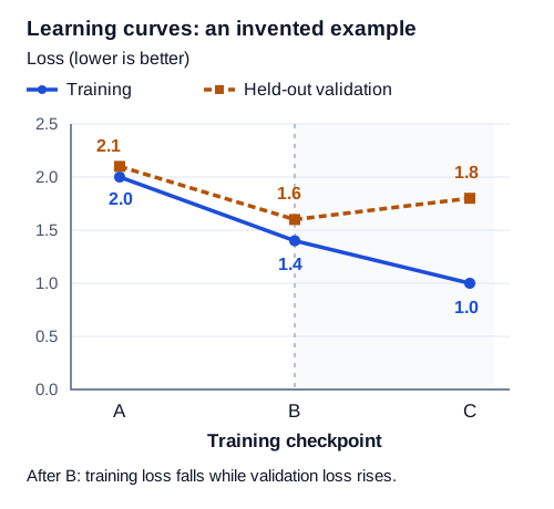
The vertical axis shows average token-prediction loss; lower means the model gave the observed targets more probability under the same scoring setup. After B, the dashed validation curve rises while training loss continues to fall. These invented measurements illustrate the pattern to investigate; they are not measurements from a real model.
Interview question: If the model already knows the next token during training, what is it learning?
Reveal the answer after explaining it aloud
Answer: The training software knows the answer, just as a teacher has an answer key. For the input “The cat,” the model must predict “sat” while its attention mask prevents it from reading “sat.” The software then measures how much probability the model assigned to “sat.” Backpropagation calculates how the weights affected that error, and the optimizer applies a weight update. The answer key grades the prediction; it is not supplied as visible input to that prediction.
20. Pretraining and post-training teach different behavior
Imagine training on books, conversations, web pages, and code. Each example asks the model to predict the next token using earlier tokens. Predicting these varied examples can teach spelling and language patterns, associations between names and facts, code conventions, and some procedures. This broad initial learning stage is pretraining.
A good continuation of a document is not always a good answer to a user. After “What is our refund policy?”, a model trained only to continue arbitrary text might write another question from an FAQ list instead of answering. To teach the desired behavior more directly, a team runs additional training on selected examples or feedback. These later stages are called post-training.
Supervised fine-tuning: demonstrate the desired response
Suppose a training example gives a support question and this policy: “Unused items can be returned within 30 days.” The desired response might be: “You can return an unused item within 30 days.” The training system increases the probability of the desired answer tokens when the model receives that input. This is supervised fine-tuning (SFT): a person or data pipeline supplies examples of the response the model should learn to produce. The loss mask determines which tokens are graded, such as the assistant answer rather than the supplied question.
The team chooses which parameters may change: all model parameters, a selected subset, or added trainable components called adapters. Section 21 works through one adapter design. SFT can teach an answer format, how to approach a recurring task, or how to respond to instructions; it can also change factual associations. What it learns depends on what the examples demonstrate and how well they cover future requests. Demonstrating correct answers during training does not check every answer the model will later generate.
Preference training: distinguish better and worse responses
For the same refund question, imagine two model responses. One accurately cites the supplied 30-day policy. The other confidently promises a refund after 90 days. A reviewer can mark the first response as better. A collection of prompts with preferred and rejected responses is preference data. It teaches a comparison between answers, instead of requiring the reviewer to author each ideal answer from scratch.
A common Reinforcement Learning from Human Feedback (RLHF) approach has two stages. First, the team trains a separate reward model to assign higher scores to responses people preferred. Second, the answer-generating model produces responses, receives scores from that reward model, and is trained to favor responses receiving higher scores. Learning from such scores is a form of reinforcement learning.
The score is an imperfect substitute for what people want. To limit unwanted changes, training often also discourages the answer-generating model from changing its response probabilities too far from a saved reference model. RLHF describes a family of methods; this two-stage arrangement is common, not a mandatory recipe for every use of human feedback.
Direct Preference Optimization (DPO) uses the preferred/rejected pairs more directly. For each pair, its training loss compares the probabilities that the model assigns to the two responses, measured relative to a reference model. Updating weights to reduce this loss encourages preference for the chosen response. The basic method does not first train a separate reward model and then repeatedly generate new responses for a reinforcement-learning stage. It still learns from the supplied preferences, so systematic mistakes or narrow preferences in the data can become model mistakes or biases.
Feedback can also come from an automated check. For a coding task, a program can run the generated code against tests and report whether they passed. Such a checker is a verifier; its result can supply a training score. Passing weak tests, however, may be possible with code that still fails the real requirement. Training toward a checker score only helps to the extent that the checker measures the desired success.
What these stages do not guarantee
Optional depth: distillation transfers behavior into a student model
Suppose an existing model gives useful answers but is expensive to run. A team can use its outputs as examples for training another model. The model providing examples is the teacher; the model trained from them is the student. This is distillation.
One approach asks the student to match the teacher's next-token probabilities. A teacher assigning three candidates probabilities [0.7, 0.2, 0.1] conveys both its preferred candidate and how strongly it favors the alternatives. Training can use that information alongside ordinary training on target tokens. Another approach simply trains on complete answers generated by the teacher. This is often called sequence-level distillation and does not require seeing all the teacher's internal token scores, or logits.
After training, the student uses its own learned weights to answer requests; it need not contact the teacher for each answer. A smaller student can cost less to run, but may repeat the teacher's mistakes or perform worse on tasks absent from its examples. The team must test the resulting student. Distillation changes how the student is trained. Quantization, explained in section 25, changes how model numbers are stored. They address different costs and can be combined. Original distillation paper.
Pretraining and post-training can improve performance without making it reliable in every situation. A model can still produce false statements, respond differently to small prompt changes, or struggle when new inputs differ from its training examples. That last change in the kinds of inputs it encounters is a distribution shift. Learning a convincing answer style does not establish a reliable solution procedure for every problem.
Evaluate the behaviors separately: can the model solve the task, follow the instruction, use the supplied evidence, and respect the application's required safety behavior? A fluent answer can succeed on style and fail on facts. Tests should measure the requirements of the actual application, not treat fluency as a substitute for them.
Read diagram source
flowchart TB
    subgraph TR["Training: update parameters using examples"]
        direction TB
        D["Training prefix tokens"] --> F["Forward calculation"]
        W[("Trainable parameters W")] -->|"Read"| F
        F --> P["Predicted token probabilities"]
        P --> L["Loss: compare prediction with target"]
        T["Actual next-token targets"] --> L
        L --> B["Backpropagation: calculate gradients"]
        B --> O["Optimizer"]
        O -->|"Update"| W
    end
    W -.->|"Save and load a checkpoint"| WF[("Deployed parameters: fixed")]
    subgraph IN["Ordinary inference: use the learned parameters"]
        direction TB
        Q["Request context"] --> G["Predict and select tokens"]
        G --> A["Generated answer"]
    end
    WF -->|"Read only"| G
Trace the arrows entering the stored parameters. In training, the optimizer writes new parameter values after the error is measured. At deployment, software loads a saved checkpoint and uses those values to calculate answers. A different prompt produces different temporary calculated numbers, or activations, while those stored parameters stay fixed during ordinary inference. The training system's target tokens go to the loss calculation; a position cannot read its own future target while making the prediction.
Interview question: Why not just pretrain on more text instead of doing SFT?
Reveal the answer after explaining it aloud
Answer: More broad text can help the model predict language, but the training examples may not show the assistant behavior we want. A policy document says what the policy is; an SFT example shows how to answer a user's question using that policy. Preference training can then favor an accurate, well-supported answer over an unsupported one. The stages supply different kinds of guidance, and each still needs evaluation.
21. Prompting, fine-tuning, and LoRA
Suppose a support application should always answer with three fields: “Decision,” “Evidence,” and “Next step.” We can put that instruction into each request, or run additional training that teaches this recurring format. The distinction is which numbers change: the request's temporary calculations or the model's stored parameters.
With prompting, the application includes “Use these three fields” in the text supplied to the model. Those extra tokens affect what the model calculates and therefore what it generates. The model's learned weights stay fixed; the temporary numbers calculated from this input, its activations, change. A model that learned to follow instructions can use that ability on the supplied format, though the instruction still needs testing on real requests.
Recognize zero-shot, few-shot, and in-context learning
An instruction such as “Convert each color name into its first letter” states the task without showing solved examples. This is zero-shot prompting: “zero” counts demonstrations in the prompt, not examples the model saw during its earlier training. Adding red → R and blue → B before asking for green → ? gives a few demonstrations, called few-shot prompting. We intend the continuation G. The model may recognize that pattern, although two examples alone do not uniquely specify every possible rule.
Using demonstrations in the current input to guide the answer is commonly called in-context learning. Here “learning” describes the model's behavior during the request. Ordinary generation does not run backpropagation or change the base weights. Supplying thousands of such pairs to a separate SFT training run would change parameters instead.
A calculator with an unchanged multiplication rule produces 6 for 2×3 and 20 for 4×5. Likewise, unchanged model weights can produce different calculated results from different input examples. This explains how behavior can depend on the prompt; it does not guarantee that the model finds the rule we intended. Few-shot language-model study.
With fine-tuning, the team runs additional training on examples of the desired behavior. The optimizer changes model parameters or added adapter parameters, and the saved result is used on later requests. This can make a recurring format more consistent or reduce repeated prompt instructions. The team must pay for training and test whether previously useful behaviors became worse, a regression, or were partly lost, often called forgetting. Teaching a format also does not supply today's refund policy unless the necessary facts are available; section 30 explains retrieving current evidence.
LoRA reduces how many parameters need to be trained
Take one learned matrix W that converts an input vector of 4096 numbers into an output vector of 4096 numbers. It has 4096×4096 = 16,777,216 stored coefficients. Full fine-tuning makes all these coefficients eligible for updates, requiring their gradients and the optimizer's additional saved state. Could we learn a useful change while training fewer numbers?
Low-Rank Adaptation (LoRA) keeps W fixed and adds a second calculation beside it. The original input still goes through W. In the new path, a learned matrix A combines the 4096 input numbers into only r numbers, and a learned matrix B expands those r numbers back to 4096. Add this new path's output to the original output. A and B form the adapter: the added component whose weights training changes. Keeping W frozen means the optimizer does not update it.
Choose r = 8. A then has 4096 rows and 8 columns; B has 8 rows and 4096 columns. Together they contain 32,768 + 32,768 = 65,536 trainable numbers, about 0.391% of the original matrix's count. The following equations describe the same calculation as a changed effective matrix W′, read “W prime.” ΔW, read “delta W,” is the added change:
The smaller path restricts what changes it can learn. Every output change must be built from combinations of the same r intermediate numbers. It cannot independently express every possible change to all 16,777,216 entries. In linear algebra, this limit is described by saying the update AB has rank at most r: at most r independent directions are available for the change. The rank-one example below makes that restriction visible. A smaller trainable component saves storage, but a particular task may need more than rank 8 for a useful adaptation.
Implementations commonly scale the update by α/r:
Here x is the input vector written as a row. xW is the original output. First xA makes the r intermediate numbers; then (xA)B expands them back to the output width. α, read “alpha,” is a chosen multiplier, so α/r controls how much of the adapter output is added. Our row-vector convention fixes the written shapes; a library using column vectors may store transposed matrices while implementing the same idea.
The original model still runs: we need its output in order to add the adapter output and measure the final error. Training also needs enough intermediate results and backward calculations to determine how A and B affected that error. Freezing W removes W's update-related gradient and optimizer-state costs, but does not remove the base model's calculation or storage. Thus “0.391% trainable parameters” does not mean “0.391% of total training memory or work.”
For a compatible deployment, software can calculate and save a merged matrix once. In the earlier unscaled example, that matrix is W + AB, written W + ΔW. When using the α/r multiplier from the inference equation above, the merged matrix must instead be W + (α/r)AB. For example, α = 16 and r = 8 require adding 2AB, not AB. The merged and separate calculations then apply the same intended change.
Later requests can use those merged weights. Other deployments keep adapters separate so several tasks can share one base model and select a task-specific adapter. If the base weights use a reduced-precision storage format, merging and rounding them again can change numerical results; the team must check that its actual serving software supports the chosen approach and preserves acceptable quality.
Optional depth: see a rank-one update and understand QLoRA
Choose a two-row, one-column matrix A = [[1], [2]] and a one-row, two-column matrix B = [[3, 4]]. Multiplying them gives the update [[3, 4], [6, 8]]. All four entries change, but the second row is exactly twice the first. It therefore supplies no second independent row pattern: this is a rank-one update.
Now follow one input. For [1, 1], the narrow calculation [1,1]A gives the one-dimensional vector [3]; expanding with B gives [3]B = [9,12]. Multiplying [1,1] by the full update matrix AB gives the same [9,12]. One intermediate number restricted the independent patterns without restricting the update to a single changed entry. Likewise, an adapter with r intermediate coordinates has rank at most r. A harder adaptation may need a larger r or adapters in different layers.
QLoRA combines this adapter training with a base model stored in fewer bits per weight. Its original method uses four-bit NormalFloat, a particular low-bit number format, plus other memory-saving techniques. Computation and adapter training use higher precision where required; “four-bit” does not mean every calculation uses four-bit arithmetic.
The base weights stay fixed while the adapter weights learn. Backpropagation may still need to follow calculations involving the base to determine how an adapter affected the loss. The system still needs activations, adapter gradients and optimizer state, and work to reconstruct usable approximate values from stored low-bit numbers. That reconstruction is dequantization. Section 25 shows a small quantization example. Compare QLoRA with ordinary LoRA using a higher-precision base, and with quantization used only for serving an already-trained model. QLoRA paper.
For a task-specific decision, continue with Fine-Tuning Strategies.
| Change | What changes for the next request? | Base weights updated by that action? |
|---|---|---|
| Rewrite a prompt or add few-shot examples | Input tokens and the activations calculated from them | No |
| Retrieve a newer document | Evidence included in the input | No |
| Save external conversation memory | Application storage; selected records may enter later prompts | No |
| Full fine-tuning | Learned model coefficients | Yes, for the trainable model parameters |
| Train a LoRA adapter | Learned adapter coefficients; the selected base stays frozen | Adapter weights change; base weights do not |
To identify the difference in practice, ask what software ran. Did the application save text or add it to a prompt? Or did a training program calculate gradients and apply parameter updates? Saved conversations could later become examples for a separate training run, but storing or retrieving them alone does not perform that training.
Interview question: When would you choose prompting, retrieval, or fine-tuning?
Reveal the answer after explaining it aloud
Answer: Identify what is missing. If the model is not told the required report format, supply an instruction or examples in the prompt. If it lacks the current policy, retrieve the policy and include it as evidence. If it repeatedly fails the required behavior despite good prompts, test whether additional training improves that behavior on separate evaluation examples. Compare the improvement with the existing system, including cost and regressions. One application can use all three approaches.
22. Generate efficiently: prefill, decode, and the K/V cache
Return to “The backup is stored in the archive. Where is the backup stored?” The application already has every token of this prompt. It can give those tokens to the model together. The answer does not exist yet: the system first selects one answer token, then uses that selected token when predicting the next. This difference between known input and unfinished output creates two phases of inference, using trained weights to calculate an answer.
Prefill processes the known prompt
The first phase, prefill, processes the known prompt through the model's blocks. At each block, every prompt position gets updated numerical representations and attention keys and values. The final prompt position produces next-token scores. After these become probabilities, the generation rule selects the first generated token. Prefill therefore does useful answer-generation work; it does not merely copy the prompt into storage.
Because all prompt tokens are available, the hardware can calculate many positions together within a layer. The causal mask still blocks future positions from each position's attention. Doing work at the same time does not grant permission to read forbidden tokens.
Decode processes the newly selected token
For illustration, suppose the first selected answer token is In. To predict what follows it, the model processes “In” at a new position through every block. This incremental phase is decode. At each attention layer, the new position's query compares with keys from the prompt and its own position. The resulting attention weights specify how to combine the corresponding values.
The prompt positions have already been processed. Must the model process them all again just because “In” was appended? For causal attention, those earlier positions could not read the new later position in the first place. Their results remain valid if the model, earlier tokens, position settings, and attention rules are unchanged. Saving their keys and values lets the next position read those results without recalculating them.
That saved collection is the key/value cache, usually written K/V cache. Each attention layer has its own collection. When the model processes In, it calculates and adds that position's key and value, then its query reads the allowed old and new entries. The cache saves repeated work on old positions; the new position still needs its own attention calculation, feed-forward network calculation, and remaining block operations.
Why cache keys and values rather than queries?
Think about which saved numbers the new calculation asks for. The query at the earlier word “backup” was used when calculating the output for that earlier position. The new “In” position does not use the earlier position's query to make its own output. It uses its own new query to compare with old keys and combine old values. Keys and values are therefore the old attention inputs worth retaining for this purpose.
An early block and a later block transform different input representations using different learned weights, so their keys and values differ. Their caches cannot simply be exchanged. The stored entries are activations: numbers calculated for this particular input. They are not copies of the learned matrices and do not form a general fact database. With RoPE position handling, a cached key normally already includes its position-dependent rotation; reusing it requires the appropriate position interpretation too.
If the user changes “backup” to “snapshot” near the start, later positions may attend differently and produce different numbers. The old cache is no longer automatically valid for those positions. Loading different weights or a different adapter can also change the calculation even when the text is identical. The server must check tokens, model and adapter identity, positions, and relevant attention settings before reusing a prefix cache. Similar-looking or similar-meaning text is not enough.
Count the generation steps carefully
Start with a short count: prefill selects token 1; processing token 1 selects token 2; processing token 2 selects token 3. If the answer ends at token 3, there is no need to process token 3 to predict a token 4. Extending this pattern, a normal request producing 100 tokens can use prefill plus 99 incremental decode forward passes. A selected stop token can likewise end generation without another forward pass for that token.
The exact scheduling changes with speculative decoding or other generation methods, but the distinction explains why “100 generated tokens” does not always mean “100 decode forward passes after prefill.”
Read diagram source
flowchart TB
    W[("Model weights: fixed")] -->|"Read"| P["Prefill: process the known prompt"]
    I["Prompt token IDs"] --> P
    P -->|"Last prompt position"| L["Scores for the next token"]
    P -->|"Store prompt K/V"| KV[("Per-layer K/V cache: activations")]
    L --> S["Select a token"]
    S --> A["Append token; display text if applicable"]
    A --> STOP{"Stop condition met?"}
    STOP -->|"Yes"| DONE["Finish"]
    STOP -->|"No: selected token is next input"| D["Decode: process that new position"]
    W -->|"Read"| D
    KV -->|"Read earlier K/V"| D
    D -->|"Append this position's K/V"| KV
    D -->|"New position predicts its successor"| L
Prefill supplies the first generated token. If generation continues, decode processes that selected token to predict the following one. Each decode pass reads the earlier cache and adds the processed position's K/V; it does not update model weights. A final selected token does not need another decode pass when the request ends.
The cache removes repeated work, not all growing work
Suppose one request has 100 cached positions and another has 1000. For ordinary dense attention, the next position must compare its query with roughly 100 keys in the first case but 1000 in the second, then combine the corresponding values. Saving the keys and values avoids calculating them again; it does not avoid reading and using them. The new position's attention work therefore grows with the number of retained positions.
Let N₀ be the number of positions already processed, T the number of additional positions actually processed, and t the current step number. At step 1 the new query reads N₀+1 allowed positions; at step 2 it reads N₀+2. Add these counts through step T. The sum sign below means to perform that addition:
Each count includes the new position itself. T counts processed positions, which can differ from the number of displayed answer tokens because prefill selected the first token. The cache eliminates much repeated computation, while the new positions' attention reads, learned matrix multiplications, feed-forward work, and output scoring remain.
| Phase | Positions being processed | Reused state | Common pressure |
|---|---|---|---|
| Prefill | Many prompt positions that are already known | A previously calculated identical compatible prefix, if available | Processing many positions together and comparing their allowed attention pairs |
| Decode | Usually one newly selected position per active answer per step | Earlier positions' keys and values from each layer | Reading weights and cached entries, coordinating many small steps, and moving data between devices |
This table describes common pressure points. The stage that actually limits speed can change with the number of simultaneous requests, model design, context length, hardware, and serving software. Measure before treating one factor as the bottleneck.
Interview question: Is the K/V cache how the model remembers yesterday's conversation?
Reveal the answer after explaining it aloud
Answer: The K/V cache saves attention calculations for already-processed input tokens so the system can reuse them on a compatible continuation. Remembering yesterday's conversation is an application decision: the product can save messages and place selected messages into tomorrow's prompt. Those saved messages, the temporary attention cache, and the model's learned weights are three separate things.
23. Calculate cache memory, then understand latent attention
Imagine a server answering 64 requests at once. It may share one set of model weights, but each different conversation usually needs its own attention cache. Longer conversations need more cached entries. The server can therefore run out of memory for requests even after the model weights fit. The number of requests being processed at the same time is concurrency. We can estimate this memory by counting what each cache stores.
Derive the ordinary K/V cache formula by counting entries
Begin with one token position in one attention layer. Each K/V head contributes one key vector and one value vector. Count how many numbers are in those vectors, then multiply by the bytes needed to store each number. Repeat that storage across all retained positions and all layers. When keys and values have the same width d_head, this counting gives:
Read each factor as something being counted:
| Factor | What it counts |
|---|---|
| 2 | One key plus one value |
| L | Number of layers storing this attention state |
| H_kv | Key/value heads per layer; grouped-query attention shares these among more query heads, so count the stored K/V heads |
| N | Token positions whose keys and values are retained for this sequence |
| d_head | Numbers in each key vector and each value vector |
| b | Bytes used to store each of those numbers |
For one token at one layer with 8 K/V heads, width 128, and two bytes per coordinate, count 2×8×128×2 = 4096 bytes. The first 2 counts keys plus values; the final 2 is storage precision. They describe different things.
For 32 layers, 8 K/V heads, 4096 positions, head width 128, and two bytes per coordinate:
That is 512 MiB for one sequence. For 64 independent conversations, each with all 4096 positions retained, multiply by 64 to obtain 32 GiB. This counts the raw keys and values only. The server also needs model weights, other temporary calculation results, memory used by the serving software, and any space lost because memory is allocated in chunks larger than the exact data.
One MiB is 2²⁰ bytes and one GiB is 2³⁰ bytes; decimal MB and GB use 10⁶ and 10⁹ bytes. Thus 512 MiB is about 0.537 GB. State the unit when reporting a capacity estimate.
Adapt the count when the stored data changes. If a key has d_key numbers and a value has d_value numbers, use d_key + d_value instead of 2 × d_head. If conversations have different retained lengths, add those lengths rather than pretending each uses the maximum. Some models keep only a recent window in certain layers; some share identical prefix entries; some use lower-precision numbers; and some store the compact representation below. Count the actual retained arrays for those designs.
Multi-head Latent Attention: store a smaller learned representation
Suppose a model would normally save many numbers per position because it has several key and value heads. Could it learn a smaller set of numbers from which the necessary key and value content can be defined? Multi-head Latent Attention (MLA) builds this choice into the attention architecture. It trains the model to use a compact internal representation, allowing a compatible implementation to save fewer cache numbers.
“Latent” means an internal numerical representation. In the equations, j labels a token position and hⱼ is the hidden-state vector representing that position as it enters this calculation. Multiplying by learned matrix W_D makes a shorter vector cⱼ; this reduction in width is a down projection. Two further learned matrices define content keys kⱼ and values vⱼ from that shorter vector. These are up projections because they expand from the compact width:
For a tiny invented example, start with hⱼ = [1, 2, 3, 4]. A chosen four-to-two matrix could add the first two numbers and the last two, producing cⱼ = [3, 7]. A chosen two-to-four key matrix could then produce [3, 7, 10, 0]. The expanded result has four entries, but they were all derived from the same two compact numbers; they cannot vary independently. Real MLA learns the down and up matrices during training instead of hand-selecting these additions. The labels D, UK, and UV mean down, key-up, and value-up.
The memory saving comes when later attention can use cached cⱼ instead of saving every expanded key and value. In the toy example, remembering [3, 7] is smaller than remembering all the expanded vectors. But an arbitrary existing model was not trained to make its keys and values follow these constraints. MLA is a model design learned during training, not a file-compression command that automatically works on any model's cache.
Even reconstructing every expanded key on every step could be wasteful. The following rearrangement shows how a compatible calculation can avoid it. The attention score compares the new position's query qᵢ with an earlier position's content key kⱼ. Substitute kⱼ = cⱼW_UK into that dot product:
The superscript T exchanges rows and columns: it turns a row vector into a column vector and also exchanges the dimensions of W_UK. Read the left side as “compare the query with the expanded key.” Read the right side as “first transform the query using the transposed key-up matrix, then compare with the compact cached vector.”
Check the equivalence with the earlier compact vector [3, 7]. Let the key-up matrix use the rules “copy the first number, copy the second, add them, output zero,” giving the expanded key [3, 7, 10, 0]. Its two coefficient rows are [1, 0, 1, 0] and [0, 1, 1, 0]. For query [1, 2, 0, 0], the ordinary dot product with the expanded key is 1×3 + 2×7 + 0×10 + 0×0 = 17. Transposing the key-up matrix makes its two rows into output columns. Applying those columns to the query gives 1×1 + 2×0 + 0×1 + 0×0 = 1 and 1×0 + 2×1 + 0×1 + 0×0 = 2. Their dot product with the compact vector is 1×3 + 2×7 = 17 again.
In this second route, the program transforms the new query once and reuses that transformed query when comparing with every source's compact vector. It does not reconstruct every expanded key. The equality comes from regrouping the same multiplications and additions; real learned key-up matrices use the same algebra with different coefficients.
The value calculation can also be regrouped: first combine compact vectors using the attention weights, then expand the resulting combined vector with the value-up matrix. This equals expanding each vector first and then adding them with the same weights, because the expansion is linear. Technical descriptions call some of these combinations projection absorption: combining compatible matrix operations so fewer expanded arrays have to be produced or stored.
Position information is an important extra part
The compact content vector is not the whole story. RoPE rotates parts of attention representations according to token position. These different rotations do not generally allow the simple matrix regrouping above to handle everything unchanged. DeepSeek's MLA design therefore separates a position-related component from the compact content pathway. Its cache retains both the compact content vector and the required rotary key state. An estimate that counts only cⱼ would miss that additional stored information.
The DeepSeek-V2 technical report describes this attention design. The exact dimensions, transformations, and performance are model-specific. Use the actual model's published architecture and serving implementation when estimating memory. The simplified equations above explain the content pathway, not every detail of a production MLA implementation.
| Technique | What it changes |
|---|---|
| GQA/MQA | Several query heads read shared key/value heads, so fewer separate K/V vectors are stored |
| MLA | Training learns a compact vector and attention transformations that can use it |
| Cache quantization | Each stored cache number uses fewer bits and approximates its higher-precision value |
| Paged cache | The server stores entries in separately allocated blocks and records where each block is located |
The first two change the attention representation; quantization changes how its numbers are stored; paging changes where storage is allocated. Their memory estimates need different inputs even when the final goal is to serve more requests.
Interview question: Why can't I estimate every model's cache using parameter count?
Reveal the answer after explaining it aloud
Answer: Parameter count measures stored learned weights. A request cache contains numbers calculated from that request, and its size depends on what each attention layer retains. I need the number of layers, K/V heads and widths—or the actual compact MLA layout—plus bytes per stored number and retained sequence lengths. Two models with similar weight counts can store very different amounts of attention state per request.
24. Long context: fitting the text is only the first challenge
Suppose a deployed model supports a combined input-and-output sequence of at most 8192 tokens. That limit is its context window under those deployment settings. It limits how much material can participate in the current sequence. It does not count how many different tokens exist in the vocabulary, how many weights the model has, or how much conversation history an application can save on disk.
With this simple 8192-token shared budget, a 6000-token prompt leaves 8192 − 6000 = 2192 tokens for the continuation. Real services can also impose separate input and output limits. Their accounting may include generated reasoning not displayed to the user, image representations, and chat-control tokens. Use the selected tokenizer and service rules when calculating the available budget.
A chat product could store years of messages, select the latest 6000 tokens for a request, and retain cache entries for the positions already processed. These are three quantities: saved conversation history, the input actually supplied now, and the attention entries currently kept for reuse. Saving an old message does not automatically put it into the model's current input.
Why full attention becomes expensive
Count comparisons in a four-token causal sequence. Position 1 can read one position; position 2 can read two; position 3 can read three; position 4 can read four. That is 1 + 2 + 3 + 4 = 10 allowed query/key pairs. For N positions, the same sum is N(N+1)/2. A full N-by-N attention score table also contains the forbidden future pairs, which the mask excludes. Either way, the number of allowed comparisons grows roughly with the square of sequence length, N².
Doubling from 1000 to 2000 positions roughly quadruples the allowed pair count. Each query/key comparison also operates on the coordinates in those vectors, and each value contribution operates on its value vector. If keys and values have the same head width d_head, the work per head therefore grows approximately as:
The symbol O, read “big O,” describes growth with problem size, not an exact count of seconds. If key and value widths differ, score comparisons grow roughly as N² × d_key and value combinations as N² × d_value. Learned projections and feed-forward networks add their own work. A direct implementation saves the entire N-by-N score table in the GPU's main high-bandwidth memory; the more efficient method below avoids keeping that large intermediate table there.
Compare that full-sequence calculation with one cached decode step. The earlier positions are already processed, so the new position makes one new query that reads roughly N retained positions. That step's attention grows roughly linearly with N. Ordinary K/V storage also grows linearly because each extra retained position adds another set of keys and values. “Quadratic full-sequence work” and “linear work for one new cached position” describe different amounts of work, so both can be true.
Different optimizations change different things
FlashAttention changes how the hardware carries out ordinary softmax attention. Instead of writing a whole score table to GPU main memory and reading it back, it processes smaller blocks of queries, keys, and values using faster working storage. As it moves between blocks, it updates the totals needed to calculate the same softmax attention result. This reduces memory traffic and large temporary storage. It still evaluates the required dense attention pairs: rearranging the work does not make the pair count linear in sequence length. Changing the order of floating-point operations can cause small numerical differences even for this mathematically exact attention computation.
Sliding-window attention changes what each position may read. For example, a position might read only its previous 128 positions, instead of all earlier positions. More generally, sparse attention evaluates a selected subset of pairs, sometimes adding designated positions that can exchange information globally. With a fixed window width w, much of the work can grow as N×w. The saving has a consequence: an arbitrary faraway sentence may no longer be directly readable from this position in this layer. Information can travel through intermediate positions across layers or through special global connections, but this is a different access pattern from full attention.
Linear attention changes the attention formula so earlier contributions can be collected into reusable summaries. To understand the storage idea, consider maintaining a running sum: a new item updates the sum without requiring all old items to be added again. Actual linear-attention methods need more structured summaries, such as sums of products involving transformed keys and values, which a new query can use. The transformation of a key or query is called a feature map.
“Linear” describes how total work grows with sequence length when the feature widths stay fixed. It does not mean every operation is a linear function. These methods usually change the query/key comparison formula, also called its kernel, or approximate ordinary softmax attention. Here a mathematical kernel is a rule for comparing two inputs, such as a query and a key. This is a different use of the word from a hardware execution kernel, the small program carrying out an operation on a processor. Linear-attention methods change or approximate the attention calculation; they do not obtain linear work merely by running every ordinary softmax comparison more efficiently.
State-space models maintain a running internal state as they process a sequence. Each new input changes that state, and the model uses the updated state to calculate outputs. Selective designs such as Mamba let the current input affect how the state is updated. This can process sequences efficiently without saving every past key/value vector in the same way as ordinary attention. However, remembering information through a state is different from directly revisiting every retained position. What the state preserves and can recall needs evaluation. A hybrid architecture mixes layer types, such as attention and state-space layers, so its memory estimate must count what each type retains.
Two research examples make the distinction concrete. Longformer selects local windows and designated global attention connections, changing which positions communicate directly. Performer uses randomly constructed feature maps to approximate softmax attention through a different calculation. Selecting fewer connections and approximating the comparison formula are different changes from FlashAttention's more efficient execution of exact attention.
Test whether a model uses the context, not just whether it accepts it
A model can accept a long prompt and still fail to find or use the relevant evidence. Test at least:
- Location: place “The backup is stored in the archive” near the beginning, middle, and end, then ask where that backup is stored.
- Interference: add a different backup ID, an outdated storage location, and unrelated paragraphs; check whether the model confuses them.
- Combination: put the original backup location in one passage and a dated migration to another location in a second passage; require using both to answer.
- Behavior: request evidence citations, then remove the needed evidence and check whether the model acknowledges that it cannot determine the answer.
- Operations: at these lengths, measure price, delay before the first token, delay while the answer streams, and how many requests the server can handle together.
Finding a single inserted fact in a long document is often called a needle-in-a-haystack test. Passing it shows useful retrieval behavior under that test, but not necessarily the ability to combine several facts or resolve contradictions. Selecting relevant passages and preparing summaries can still help when the model accepts a large window, provided those steps preserve the evidence the answer needs.
Interview question: Does FlashAttention solve the long-context problem?
Reveal the answer after explaining it aloud
Answer: FlashAttention reduces the traffic and temporary storage needed to calculate exact attention. It still calculates the required pairs, so processing a whole dense-attention sequence still has roughly quadratic attention arithmetic. Even if the computation fits and runs quickly, a separate test must check whether the trained model actually finds and uses the relevant distant evidence.
25. Model size, numerical precision, and arithmetic cost
Suppose a model is described as “7B.” B means billion, so the model has roughly seven billion learned parameters. This counts stored adjustable numbers, not facts or tokens. A four-row, two-column learned matrix has eight parameters whether it processes three input rows or three thousand. Processing more input reuses the same weights while creating more temporary results and cache entries. Keep these two counts separate when estimating memory.
Start a weight-memory estimate with bytes per parameter
Start with the simple rule number of stored parameters × bytes per parameter. A byte contains eight bits, and a bit stores one binary digit. Different numerical formats use different numbers of bits for each model number. For a dense model with seven billion parameters, this gives:
| Weight format | Approximate bytes per parameter | Raw weight storage |
|---|---|---|
| FP32: 32-bit floating-point numbers | 4 | 28 GB |
| FP16 or BF16: two 16-bit floating-point formats | 2 | 14 GB |
| INT8: 8-bit integer codes | 1 | 7 GB |
| INT4: 4-bit integer codes, packed two per byte | 0.5 | 3.5 GB |
These are decimal GB; 14 GB is about 13.0 GiB. They count only the raw weight data. A real deployment also stores information needed to interpret quantized numbers, may keep some arrays at higher precision, and needs request caches, temporary working arrays, and memory for the serving software. Training additionally stores gradients, intermediate forward results, the optimizer's saved history, and sometimes higher-precision copies of weights. A GPU that fits the raw weights can still lack enough memory to run the desired workload.
Optional calculation: why training memory exceeds weight memory
Consider one illustrative training implementation using an Adam-style optimizer. For each parameter, it stores a two-byte weight used in forward calculations, a two-byte gradient, and a four-byte master weight copy used to retain more precision during updates. It also keeps two four-byte optimizer arrays: a running average of gradients and a running average of their squares. These averages are often called optimizer moments.
Add these arrays: 2 + 2 + 4 + 4 + 4 = 16 bytes/parameter. For 7B parameters, that is 112 GB, or about 104.3 GiB, before the intermediate results and other working memory. If the gradients instead use four bytes, the same named arrays use 18 bytes per parameter. Other implementations omit the master copy or use different precisions. Count what the implementation actually stores; 16 bytes is an example, not a universal requirement.
The memory for intermediate calculated results, or activations, also depends on how many examples are processed together, their token lengths, the width and number of model layers, and what backpropagation needs to reuse. Activation checkpointing saves fewer results and recalculates others later. Sharding distributes arrays across devices, so one GPU need not store every parameter, gradient, or optimizer array; the devices then communicate the information required by the calculation. LoRA reduces which parameters need gradients and optimizer state, while the base model weights and necessary intermediate results still occupy memory.
Floating-point formats represent numbers using a sign, a scale called the exponent, and digits carrying precision. Think of scientific notation such as 1.23 × 10⁵: changing the exponent changes the range of magnitudes, while keeping more digits in 1.23 improves precision. Computer floating-point formats use binary rather than this decimal example. FP16 and BF16 both use 16 bits, but BF16 assigns more to the exponent range and fewer to precision than FP16. It can represent a wider range of magnitudes with coarser precision.
INT8 and INT4 instead store small integer codes that a quantization scheme maps to approximate model values. Knowing the bit count tells us storage size, but does not fully specify the mapping or how fast the hardware's implementation can use it.
Quantization trades precision for smaller representation
Suppose the model has a weight 0.26, but our storage scheme can represent only multiples of 0.1. Divide 0.26 by the chosen scale 0.1 to get 2.6, then round to integer code 3. Store 3 along with the scale information. When the calculation needs the approximate weight, reconstruct 3 × 0.1 = 0.3. The storage decision changed 0.26 into 0.3, an error of 0.04. Mapping values to such a restricted set is quantization.
Real schemes choose how many values share a scale: perhaps a whole array, an output channel, or a smaller group. They may also use an offset, which shifts the range represented by integer codes, or clipping, which limits extreme values to the representable range. Calibration runs representative examples to help choose suitable ranges and settings. Other schemes use specialized number formats. All require deciding which approximations are acceptable. Fewer stored bits can reduce memory and data movement, while rounding and range limits can change the model's answers.
There are two common times to introduce these approximations. Post-training quantization (PTQ) starts from an already-trained model and converts it, often using calibration examples. Quantization-aware training (QAT) includes the effect of reduced precision during training, either simulated or actually used, so weight updates can adapt to it.
A single deployment can mix formats. Stored weights might use four bits while intermediate results, the K/V cache, and accumulators—numbers holding running sums during multiplication and addition—use more bits. “A 4-bit model” therefore often describes weight storage, not every operation. Test the chosen configuration for answer quality, important rare errors, speed, total work served per second, and memory. Specialized device routines, called kernels, determine whether the hardware can turn smaller stored numbers into faster execution.
Estimate compute, but state the assumptions
In a dense matrix multiplication, each used weight contributes roughly one multiplication and one addition. Counting both as floating-point operations gives roughly two operations per used parameter per token. If most of a dense model's P parameters participate in that way, we get this rough estimate for one forward calculation:
P is parameter count, and FLOPs means floating-point operations. For P = 70 billion, 2P is about 140 billion operations, or 140 GFLOPs per token; G means billion. Processing 100 token positions with this approximate amount of forward work would require about 14 trillion operations. This is an estimate of work, not seconds.
It leaves out terms such as the attention comparisons over context. It also assumes parameters are used in the counted way: selecting an input embedding row is not a full dense matrix multiply, and one shared input/output weight array can play different computational roles. Use 2P for an initial estimate and then account for the actual architecture and request lengths.
A dense linear layer performs one matrix multiplication in the forward pass. Backpropagation needs two related calculations: how the error changes with the layer's input values, and how it changes with the layer's stored coefficients. These are two more matrix multiplications, each with roughly the same arithmetic count as the forward multiplication. Thus training these layers costs approximately three forward passes' worth of matrix work: one forward calculation plus two backward calculations.
Using the earlier estimate of 2P forward operations per token gives 3 × 2P = 6P training operations per token. If D is the number of training tokens processed, multiply by D:
The estimate is not exact: long-context attention adds work, activation checkpointing repeats some work, and architectures that run selected components can change which parameters participate. The implementation also has work outside these matrix calculations.
Keep amount and rate separate. FLOPs count operations, like counting distance traveled. FLOP/s counts operations per second, like a speed. Dividing work by a hardware's advertised maximum rate is not a reliable latency prediction if the hardware spends much of its time waiting for data or communication. Section 28 works through that bottleneck.
Interview question: Can I compare models just by parameter count?
Reveal the answer after explaining it aloud
Answer: Parameter count tells me how many learned numbers are stored, which helps estimate weight memory. It does not tell me whether the model learned the required task or how expensive a request will be. I would also check the training data and objective, which model components run per token, context handling, numerical precision, and measured performance on the intended requests. A resource estimate and a quality comparison answer different questions.
26. Mixture of Experts: give each token selected FFNs
In an ordinary dense layer, every token position goes through the same feed-forward network, or FFN. Imagine instead providing four alternative FFNs, each with its own learned weights, and choosing two of them for each position. The selected networks process that position's input vector, and their results are combined. This arrangement is a Mixture of Experts (MoE). A small learned calculation called the router makes the selection.
An expert here is one of those FFNs. It transforms numbers inside a model layer; it is not a complete chatbot answering its own question. Training may cause experts to become useful for different input patterns, but the label “expert 3” does not assign it a human profession such as medicine.
Think of a workshop that sends each work item to selected stations. The router is the dispatcher, each expert is a processing station, and the layer combines the selected stations' results. The analogy explains selection and possible queues. In the actual model, the work item is a position's hidden-state vector and the dispatch decision is also a learned numerical calculation. If many items choose the same station, it can become overloaded while other stations sit idle.
Walk through one routing decision
Give the router one position's input vector. Suppose it calculates the four scores [2.1, −0.4, 1.7, 0.2], one for each expert in order. A top-2 rule means “select the two highest scores,” so this position goes to experts 1 and 3. Experts 2 and 4 do not process this position.
We also need a rule for how much each chosen output contributes. In this example, apply softmax to only the selected scores 2.1 and 1.7. This turns them into positive combination weights that add to one: about 0.598688 and 0.401312. Suppose expert 1 produces [2, 0] and expert 3 produces [0, 5]. Multiply each output by its combination weight and add matching coordinates:
For the first output coordinate, the calculation is 0.598688×2 + 0.401312×0. For the second, it is 0.598688×0 + 0.401312×5. Real MoE designs can use different scoring and combination rules, and some include shared experts that run for every position. The numerical example teaches one routing choice, not a universal rule.
The important sequence is: score experts for this position → select a subset → run those networks → combine their outputs. The next position can select a different subset.
Read diagram source
flowchart TB
    X["Input vector for one position's feed-forward calculation"]
    X --> R["Router: score experts; select the highest 2"]
    X --> D["Send the same input vector to selected experts"]
    R -->|"Selection"| D
    D --> E1["Expert 1 output: [2, 0]"]
    D --> E3["Expert 3 output: [0, 5]"]
    R -.->|"Not selected"| SK["Experts 2 and 4: not run"]
    E1 -->|"Multiply by 0.598688"| S["Add selected weighted outputs"]
    E3 -->|"Multiply by 0.401312"| S
    S --> Y["Combined feed-forward update: about [1.197, 2.007]"]
Follow the two paths in the diagram. The router's scores decide where to send the input and how to combine results. The experts receive the original FFN input vector, not the router scores themselves. The next token may select different experts. This arrangement replaces an FFN component of a Transformer block; the block still needs its attention calculation.
Total parameters and active parameters answer different questions
Imagine 8 experts, each containing 1 billion learned parameters, plus 2 billion parameters in components shared by all tokens. The whole model stores 8×1B + 2B = 10B parameters. If each token runs two experts, its calculation uses about 2×1B + 2B = 4B parameters. The first count is total parameters; the second is active parameters per token. They answer how much is stored and how much participates in one token's calculation.
A documented larger example is DeepSeek-V3: its report specifies 671 billion total parameters and 37 billion activated per token. These two counts describe different aspects of the same model.
This allows the model to store a larger collection of learned transformations while using a subset for each token. But the server cannot assume it only needs to make 4B weights available. Different tokens can choose different experts, and a group of simultaneous requests may collectively select every expert. The deployment must decide where to keep the full model: loaded on devices, sharded across devices, or offloaded to another memory tier and transferred when needed. Moving weights has costs too.
The operational difficulties come from routing
Suppose 90 out of 100 positions select expert 1 while only 5 select expert 4. Expert 1 has much more work. This is load imbalance. Training can encourage a more useful spread of selections, and serving software must schedule the resulting work. If expert 1 lives on another GPU, software must also send the selected positions' input vectors there and return their outputs.
Some designs reserve room for a limited number of positions per expert in each batch, a group of positions processed together. If more positions select that expert than fit in its reserved capacity, the system needs an overflow rule. It might omit those positions from that expert's contribution, send them to another expert, or use a dropless design that handles all selections with different storage and scheduling costs. Persistently sending most positions to a small subset is called router collapse. It can leave other experts undertrained and hardware underused.
One training approach adds an auxiliary balancing loss: an extra penalty, alongside the main prediction loss, that discourages an undesirable distribution of expert selections. Different models use different balancing mechanisms. The DeepSeek-V3 technical report describes a strategy called auxiliary-loss-free balancing for much of this purpose and also a sequence-wise auxiliary balancing loss, which adds a balancing signal within individual sequences. The model therefore cannot accurately be described as having no auxiliary balancing term at all.
When experts are on different devices, sending inputs and collecting results takes time beyond the experts' arithmetic. A request routed through an overloaded expert may wait especially long. This affects tail latency, the slow end of the request-time distribution. A small active parameter count can therefore coexist with expensive data transfers and slow requests.
Interview question: Why can a 10B MoE with 4B active parameters cost more to serve than a 4B dense model?
Reveal the answer after explaining it aloud
Answer: The MoE still needs all 10B weights available somewhere, because different tokens can select different experts. It also calculates routing decisions, can queue behind overloaded experts, and may send input vectors and results between GPUs. The 4B active count describes which weights participate for one token; it leaves out those storage and coordination costs. I would compare actual request quality, memory, and speed on the intended workload.
27. Training-optimal, serving-optimal, and inference-time compute
Suppose a team wants an accurate assistant at a manageable cost. It could train a larger model, train a smaller model on more examples, or keep its current model and check several candidate answers for each request. These spend computation at different times and for different purposes. “Which model size is best?” needs a specified budget and objective before it has a useful answer.
Decision 1: divide a fixed training budget between size and data
Imagine having a fixed number of GPU-hours for training. A larger model performs more work on each token, so that budget may allow it to see fewer training tokens. A smaller model can process more tokens for the same budget and may achieve a better final score. Choosing the model size and amount of data that work best together under that budget is the question studied by compute-optimal scaling. “Compute” here means the computational work available for training.
The Chinchilla study found that some earlier large models had seen too little data relative to their size to make the best use of their training budget. Under its studied conditions, the preferred numbers of parameters and training tokens grew roughly together. Its 70B-parameter model trained on 1.4T tokens: 1.4 trillion / 70 billion = 20, giving the familiar roughly 20 training tokens per parameter. This is a result and reference point from that study, not a rule that every model, dataset, or training method should use that ratio. Chinchilla paper.
A scaling curve summarizes how measured performance changes as size or data increases across training runs. It describes a trend under those runs' conditions. Duplicate removal, the mixture of subject areas, example quality, context length, and the update procedure still affect results. Repeating poor examples increases the token count without necessarily providing equally useful learning.
Decision 2: minimize cost over the model's useful lifetime
Now change the budget question. The team pays for a training run and then pays to answer many future requests. A smaller model that takes extra training to reach the required quality could still save money over its lifetime if each later request costs less. Serving means running the trained model for users, so serving-optimal choices include this future workload.
Suppose the extra training costs 100,000 currency units and saves 0.01 unit on every later request while maintaining acceptable quality. Divide the extra cost by the saving: 100,000 / 0.01 = 10,000,000 requests. At that break-even point, the request savings equal the extra training cost. This simple example excludes other costs, but explains why the cheapest way to finish one training run need not give the cheapest model to operate for years.
Meta reports more than 15 trillion pretraining tokens for its Llama 3 8B and 70B models. Those are much higher token-to-parameter ratios than the Chinchilla reference above. They illustrate a different allocation choice when building models for later use. The example does not prove that either ratio minimizes every application's lifetime cost. Llama 3 report.
Decision 3: spend more computation on a particular answer
The third decision happens after training. For one difficult request, the application can allow more generated reasoning, ask for several candidate solutions, run tools, or check and revise an answer. This extra work while solving the request is inference-time compute. It spends additional operations on this answer instead of changing model size or running another weight-training stage.
For example, the application might ask for four candidate programs, run tests on each, and select one that passes. It pays for four generations and the tests. This can help if the candidates include better solutions and the tests identify them. If the tests miss important requirements, all four candidates could be wrong in the same untested way. Extra work then raises cost and waiting time without providing the needed improvement.
The team should measure how task success changes as it allows more candidates or checks, counting the cost of failures and verification too. This produces a quality-versus-cost comparison for the actual task. The length of the visible explanation is not that measurement: a long answer can still contain the same mistake, and some tasks do not benefit from extra attempts.
| Decision | Budget being allocated | Main comparison | Evidence needed |
|---|---|---|---|
| Training-optimal size/data | Work available for one training plan | Train a larger model on fewer tokens, or a smaller one on more tokens | Compare performance on separate evaluation examples after controlled training runs |
| Serving-optimal lifetime cost | Training cost plus the cost of future requests | Pay for extra training now to reduce later request cost | Required answer quality, expected request count, and measured cost per request |
| Inference-time computation | Extra work allowed on the current request | Generate and check more candidates or spend longer on one attempt | How much verified task success improves per added cost and waiting time |
For related architecture choices, see Model Taxonomy; for economic decisions, see Cost Optimization Playbook.
Interview question: How would you choose between a larger model and more inference-time checking?
Reveal the answer after explaining it aloud
Answer: I would compare both approaches on the same tasks and the same definition of a correct result. I would count the entire waiting time and cost, including generated candidates, tools, checks, and failed attempts. A smaller model plus reliable tests may be attractive for tasks whose answers can be checked. If the checker accepts important mistakes, its low apparent cost may be misleading. The decision needs measured success, not just model size or answer length.
28. Why an LLM service can be slow even when the model is correct
A user sends a question and waits for an answer. During that wait, the application may queue the request, collect instructions and saved history, search documents, run the model, call a tool, and transmit the output. Even a mathematically correct and fast model calculation can sit inside a slow application. To improve speed, first measure where the time goes.
Separate first-token time, streaming speed, and throughput
Start a timer when the request begins. The delay until the first generated token arrives is time to first token (TTFT). Depending on the measurement boundary, it includes work such as queueing and prefill. Once generation is streaming, measure the gaps between later tokens: this is inter-token latency. Across the whole server, count completed requests or generated tokens per second: this is throughput. State which count is being reported.
For example, the first token arrives after 0.4 seconds. The next 99 arrive 0.02 seconds apart. Receiving 100 tokens therefore takes approximately 0.4 + 99×0.02 = 2.38 seconds. After the first token, that one answer streams at 1 / 0.02 = 50 tokens per second. If the server streams several answers at once, its total tokens per second can be higher than this single user's rate.
Waiting briefly to collect more requests into a batch might increase the server's total work per second while delaying an individual user's answer. Measure the whole request-time distribution under realistic load. The median is the middle observed latency. p95 is the latency at or below which 95% of requests fall, helping expose slower cases in the tail. One fast demonstration does not reveal what happens when many users arrive together.
Decode often has to move a lot of bytes for little work
Suppose a GPU processes one new token for only one or a few requests. It may need to read a large fraction of the model weights from memory for that small amount of output. It also reads the relevant K/V entries. The calculation units can spend time waiting for these numbers to arrive. This is a memory-bandwidth bottleneck: how quickly bytes can move limits progress more than the maximum arithmetic rate does.
For a hypothetical step, assume 32 GB must be read and sustained usable bandwidth is 1 TB/s, or 1000 GB/s in decimal units. The reads alone take at least 32 / 1000 = 0.032 seconds under ideal conditions. This is a lower bound for those assumed bytes, not a full request-time estimate. Reading cache data, communicating between GPUs, and running other operations can add work. Reusing the same loaded weights across several requests in a batch can reduce the weight-reading cost per generated token.
Therefore, a GPU's advertised peak floating-point operations per second does not directly tell us its generated tokens per second. The actual request must supply data fast enough to keep those arithmetic units busy.
Continuous batching fills available capacity
Imagine requests A, B, and C generating together. A finishes after 10 output tokens; B and C each need 100. Waiting for the whole original group to finish would leave A's available capacity unused. With continuous batching, the serving scheduler can remove completed A and admit waiting request D while B and C continue, when memory and scheduling rules allow. This helps keep the hardware busy despite different request lengths.
The scheduler is the software choosing which work runs next. It must balance available memory, fair waiting times, and ongoing streaming speed. Processing a very long new prompt can compete with the small decode steps for existing answers. Grouping more work can spread one weight read across several requests, but admitting too much work can cause long queues or consume too much cache memory. Measure both throughput and user waiting time when changing batching rules.
Chunked prefill divides a long prompt's processing into smaller scheduled chunks. Later chunks retain access to the earlier prompt's cached keys and values; chunking does not create independent prompts or shorten the intended attention context. The scheduler can interleave these chunks with decode work for answers already streaming, reducing the time those answers wait behind one large prefill. Smaller chunks may protect inter-token latency but add scheduling overhead or delay completion of the new request's prefill. The useful chunk size depends on the workload and hardware, so evaluate both time to first token and streaming latency. vLLM's chunked-prefill explanation.
Paged cache reduces allocation waste
Suppose a cache slot holds one token position's retained data. Two conversations currently need 18 and 31 slots, for 49 used slots altogether. Reserving a single 64-slot region for each conversation occupies 128 slots, leaving 79 unused. Instead, allocate small blocks of 16 slots as needed. Each conversation needs two blocks, so the server reserves 64 slots total, with only 15 unused in this example.
This is the storage idea behind a paged K/V cache. The serving software records a table saying which memory block holds each range of a conversation's token positions. The blocks need not sit next to one another in physical memory. The model can still read tokens in their correct sequence order because the table locates their data. Allocating smaller blocks can reduce wasted or unusable gaps, called fragmentation.
Two compatible requests can sometimes share unchanged cache blocks for the same prefix. If one branch needs to change a shared block, the system must preserve the other branch's data, often by giving the changing branch a separate copy first. This is copy-on-write: share while the contents remain identical, copy when an independent write requires it.
Paging changes where the entries are stored and how unused capacity is managed. Each token's key/value representation is still the same size unless another technique changes it. “Paged” also does not automatically mean data moves to disk; these cache pages can remain in GPU memory.
Three caches or scheduling ideas, three different jobs
| Technique | What is reused or shared | What must remain valid |
|---|---|---|
| Continuous batching | Several requests share scheduled use of the hardware | Each request's tokens, cache, and stopping conditions remain separate and correct |
| Prefix caching | Saved keys and values for an already-processed beginning of a request | The prefix tokens, model and adapter weights, positions, and relevant settings match |
| Answer caching | The application returns a previously saved answer | The answer is still appropriate for the question, current evidence, and this user's permissions |
For example, “Where is the backup stored?” and “Which location holds the backup?” may mean similar things but have different token sequences and attention calculations. Their K/V cannot automatically be shared. Even an identical question cannot safely reuse an old answer if the location or the user's access to the underlying document changed. Each cache needs an explicit rule for when reuse remains correct.
More than one GPU introduces placement choices
If the model cannot fit or run efficiently on one GPU, the deployment can divide work across several. The division determines what data must travel between them:
- Tensor parallelism: divide a large matrix calculation. For example, each GPU computes a subset of an operation's output coordinates, then the devices exchange or combine results required by later operations.
- Pipeline parallelism: place successive groups of layers on different GPUs. One device processes the earlier layers and sends their output to the device holding later layers. Multiple pieces of work can be scheduled at different stages of this pipeline.
- Expert parallelism: place different MoE experts on different GPUs. Send each selected input to the device holding the chosen expert and gather its output.
Another option is to keep multiple model copies, called replicas. In training data parallelism, replicas process different examples, then combine their gradients so their parameter updates stay coordinated. During serving, independent replicas can answer different requests with the same saved weights without combining training gradients, because ordinary requests do not update those weights.
Adding GPUs can provide enough memory or handle more requests, but it adds communication. A pipeline stage can also wait for a slower stage, and very small decode steps may spend a large fraction of time coordinating devices. Measure the real request lengths and concurrency on the actual interconnect, the hardware links carrying data between devices, before promising lower latency.
Speculative decoding: propose quickly, verify with the target
Suppose a smaller, cheaper draft model proposes the next four tokens. The larger model whose answers we want, the target model, can evaluate those proposed positions together. If several proposals are accepted, one target evaluation advances generation by several tokens instead of only one. This is the idea of speculative decoding; proposal methods do not always require a separate small model.
For exact speculative sampling, acceptance is a probability calculation. Consider just one next-token sampling decision, with two possible tokens, tea and coffee, after the same supplied prefix. Suppose the draft assigns probabilities [0.8, 0.2] to [tea, coffee], while the target assigns [0.6, 0.4]. The draft proposes a token by sampling its own probabilities. We need to correct its excess preference for tea while preserving the target's intended choices.
For a proposed token, divide its target probability by its draft probability and cap the result at 1. This is the probability of accepting that proposal. A proposed tea is accepted with probability 0.6/0.8 = 0.75; a proposed coffee is always accepted because 0.4/0.2 = 2, which is capped at 1. If tea is rejected, choose from the correction distribution: subtract draft probabilities from target probabilities, replace negative differences with zero, then divide by the remaining total. Here the differences are [−0.2, 0.2], which become [0, 0.2] and then [0, 1]. The correction therefore chooses coffee.
Now count the final outcomes. tea is proposed 80% of the time and accepted 75% of those times, giving 0.8×0.75 = 0.6. coffee is either proposed directly or selected after rejecting tea, giving 0.2 + 0.8×0.25 = 0.4. These are exactly the target's probabilities. Acceptance is not a judgment that a phrase sounds good: the acceptance and correction calculations preserve the intended distribution.
For a proposed sequence, the program applies the corresponding checks in order using the appropriate prefix at each position. After rejecting one proposal, it cannot simply retain later proposals that assumed that rejected token was part of the prefix. The exact algorithm manages that stopping point and correction so the final sampling probabilities still match the target model's intended procedure.
The extra proposal work pays off only if enough proposed tokens are accepted and target verification is efficient. A poor draft or expensive verification can make the system slower. The speedup also depends on batch size and hardware. Approximate variants may relax the exact probability guarantee; then the team needs to state and evaluate how the generated distribution or answer quality changes.
Interview question: How would you investigate a slow product?
Reveal the answer after explaining it aloud
Answer: I would trace representative requests and measure the time spent waiting in queues, fetching evidence or running tools, processing the prompt, generating later tokens, and delivering the answer. Then I would inspect the busiest stage: request lengths, cache usage, batching, memory reads, or GPU communication may explain it. I would change the measured bottleneck and check whether total cost, answer quality, median latency, and slow-case latency improved under realistic load.
For the deployment mechanisms and workload measurements, continue with Serving Infrastructure and Observability.
29. How images and audio enter a model built from vectors
Consider asking “Which rack contains the server?” with a photo attached. A model cannot multiply raw human meanings. It needs numerical input describing both the words and the image. The Transformer operations can process vectors even when those vectors came from image regions or audio segments rather than text-token lookups.
For text, the tokenizer produces IDs and the embedding table supplies their initial lists of numbers, or vectors. An image-processing component can instead calculate vectors from image regions. An audio-processing component can calculate vectors from time segments, or turn audio into learned discrete units with IDs. Text, images, and audio are different modalities, meaning kinds of input or output. A multimodal model works across more than one kind. Training must teach the system how these numerical inputs relate to the answers users want.
A concrete image-patch example
Take a 224 × 224-pixel image and divide it into nonoverlapping 16 × 16 patches:
There are 196 patches. In an RGB image, each pixel has three channel values for red, green, and blue. One 16-by-16 patch therefore contains 16×16×3 = 768 numbers. A simple design writes those values into one ordered vector, then multiplies that vector by a learned matrix to obtain the desired vector width. This is a patch projection. A vision encoder, the learned component that processes images, may then run many additional transformations before its outputs reach the language model.
To identify which rack contains the server, the model also needs information about where patches came from. The contents of a patch alone do not say whether it came from the upper-left or lower-right corner. The model design must preserve location through the ordering of inputs or position mechanisms, just as text processing needs information about token order.
There are different ways to connect the image component to the language component. In the first diagram, a learned projector converts image vectors to the width required for joining the language model's input sequence. In the second, image states remain separate, and cross-attention lets queries from the text-side calculation read keys and values derived from them. Audio and video also require time information: for example, which video frame and spoken word occurred together. Choosing which frames to process and how to align sound with images affects what the model can use.
Connection A: insert visual vectors into the language sequence.
Read diagram source
flowchart TB
    I["Image patches"] --> E["Vision encoder"]
    E --> P["Projector: match the required vector width"]
    P --> V["Visual vectors"]
    T["Text token embeddings"] --> S["Combined input sequence"]
    V --> S
    S --> L["Language-model blocks"]
Connection B: let decoder queries read separate visual states.
Read diagram source
flowchart TB
    I["Image patches"] --> E["Vision encoder"]
    E --> KV["Visual keys and values"]
    T["Hidden-state vectors for the text so far"] --> Q["Queries calculated from those text representations"]
    Q --> C["Cross-attention"]
    KV --> C
    C --> U["Update text representations using visual contributions"]
Follow the concrete data in each diagram. In connection A, vectors calculated from the image become entries in a combined sequence beside text embeddings. In connection B, text-side queries calculate how to combine separately stored visual values. The diagrams describe where the numbers go. They do not yet say which weights training will change; that is a separate choice below.
Equal vector width is necessary for some connections, not sufficient for understanding
Suppose both the image component and the text embedding table output 4096 numbers. Their shapes may now fit the same input operation, but equal vector width does not make the representations mean the same thing. Training still needs examples connecting visible equipment with relevant words and tasks. Teams can train components together or in stages to establish this relationship. Making two plugs physically fit is a useful analogy for matching dimensions; it does not by itself teach the system how to interpret the signal.
Descriptions such as “native multimodal” may refer to more integrated training or architecture, but the phrase does not specify one design. A system may still use separate image and audio components or connecting adapters. To estimate quality or cost, read the actual architecture and evaluations rather than inferring them from that label.
Separate the connection from the training policy
Suppose the team already has a useful vision encoder and language model. It might begin by changing only the projector connecting them. The encoder and language model are frozen: the optimizer does not change their parameters in this stage. The projector is trainable: its parameters can receive updates. Later training might also change selected language-model weights. Here are three illustrative choices:
| Illustrative stage | Vision encoder | Projector | Language model | What the stage can teach |
|---|---|---|---|---|
| Projector alignment | Frozen | Trainable | Frozen | Teach the connecting matrix to turn image outputs into inputs that help the fixed language model predict the required text |
| Visual instruction tuning | Frozen | Trainable | Trainable, or selected adapters trainable | Use examples of image-and-text questions with desired responses to improve instruction following |
| Broader joint tuning | Selected or all parts trainable | Trainable | Selected or all parts trainable | Let more components adapt, then test whether the changes also harm previously useful behavior |
These are possible policies, not a required sequence. The first two resemble stages in Visual Instruction Tuning. The third illustrates choosing to update more components. A cross-attention architecture can choose differently: Flamingo learns connecting components while keeping pretrained vision and language models frozen.
Freezing weights does not always remove the component's backward calculation. If the projector's output passes through a frozen language model before producing the loss, training still needs to calculate how changing that projector output would affect the loss through those operations. Backpropagation may therefore run through a frozen component to reach an earlier trainable component, even though the frozen component's own weights are not updated.
The 196-patch example counts this particular image split. It does not tell us how many billable tokens an API assigns to every uploaded image. Real systems may resize an image, crop regions, split it into tiles, or combine several patch representations into fewer outputs through pooling. Different resolutions, frame counts, and audio lengths therefore affect work and context according to the chosen design and the service's accounting rules.
Interview question: Does a multimodal LLM turn every image into a text caption before reasoning?
Reveal the answer after explaining it aloud
Answer: No. An image encoder can calculate vectors describing image regions, and the language calculation can use those vectors directly through a connecting projection or cross-attention. A system could instead generate a caption first, but a short caption might omit a detail needed by the question. Handling image-derived numerical representations, with training that connects them to the task, does not require first translating the whole image into prose.
30. What the model knows, what the application supplies, and why errors remain
Suppose the model can often answer “What is the capital of France?” without being given a document. During training, its weights changed in ways that help it predict relevant language, including factual associations such as France and Paris. These learned patterns can also support grammar, writing styles, and procedures. But the weights do not expose a reliable database record labeled “source of this fact,” with an address and citation the application can always retrieve.
If the model applies a learned pattern to a new combination of inputs, that is generalization. For example, it may follow a familiar formatting rule on a sentence it has never seen. It can also memorize particular training sequences and sometimes reproduce them. These behaviors can coexist in one model. A new-looking answer does not prove that the model cannot reproduce training material, so teams must consider privacy and permitted data use when selecting training data and evaluating outputs.
Retrieval supplies evidence at request time
Consider the question “Can I return this item after 20 days?” The application can search the company's current policy collection, find “Unused items may be returned within 30 days,” and place that passage beside the user's question in the model's input. The model then generates an answer using the supplied policy. This pattern is retrieval-augmented generation (RAG): retrieval finds evidence, and generation uses it in the request context.
The search step changes the input to this request; it does not run an optimizer update on the model's weights. It can therefore supply current or private information without retraining. Each step can still fail. Search might miss the policy or find an obsolete version. Splitting documents into small passages, called chunking, might separate a return rule from its exceptions. Even with the right passage present, the model might apply it incorrectly. Evaluate both finding the evidence and using it.
One way to search is to calculate an embedding vector for the question and a vector for each passage, then compare those vectors using a chosen similarity rule. A retrieval embedding model is trained to make such comparisons useful. Its output represents a whole query or passage for search; it is not simply one token's row from the answer-generating model's input embedding table.
The application can combine this vector search with keyword matching, metadata filters such as document date, and reranking, a second model or scoring step that reorders retrieved candidates. The query and passage representations must be compatible. Two unrelated models producing vectors of 768 numbers do not necessarily use those coordinates in comparable ways. When creating or rebuilding the search index, the stored search structure, record the encoder versions and text preparation rules together so future queries are compared with appropriately produced document vectors.
Tools perform actions outside the model
Suppose the answer requires today's shipment status. The model can generate a structured request containing a tool name and arguments, such as an order ID. The surrounding application checks whether that request is valid and authorized, calls the shipment service, and returns the actual result as new input. The model can then explain it. The model produces the requested action description; the application executes the action through a program or API, an interface for one program to request work from another.
The application must check the order ID, permission to read it, whether the service failed, and whether the requested tool would change anything outside the conversation. Those external changes are side effects. A well-formed tool request does not prove that a shipment lookup or money transfer succeeded. The answer must rely on the actual execution result.
External memory is stored application data
A product might save “the user prefers concise answers” in a profile and include that sentence in later prompts. The assistant can then adapt its response across sessions without any weight update. This external memory is application data. The full saved transcript, a shortened summary, the search index, and the currently usable K/V cache each serve a different purpose. The product must decide how long to retain each and when its contents are still appropriate to use.
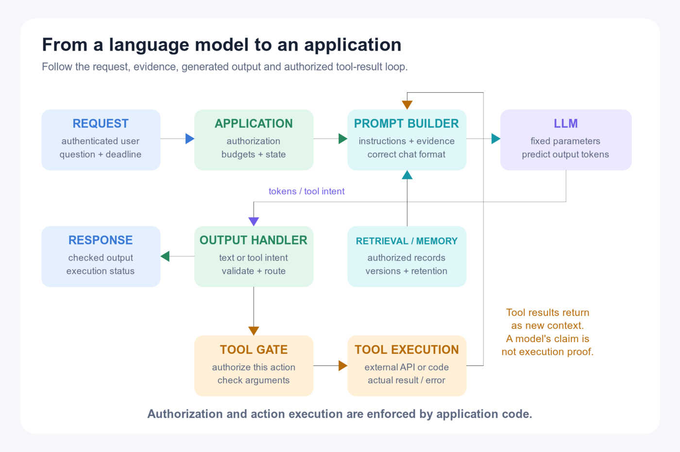
Why next-token prediction can produce a false statement
For the application designs around the model, see RAG Fundamentals and LLM Evaluation.
Suppose the model has no reliable evidence about whether the backup was migrated this morning. It can still assign probabilities to possible answers, and “in the archive” may sound plausible given earlier text. Selecting a plausible continuation does not establish the current storage location. A model may also reproduce inconsistent training information, follow a misleading assumption in the question, or make a mistake while combining facts. These can produce a fluent but false statement, often called a hallucination.
Softmax can correctly turn the model's scores into probabilities even when the highest-scoring sentence is false. Lowering sampling temperature may simply make the system choose that same false sentence more consistently. Adding more text helps only if it includes useful evidence and the model uses it correctly; more tokens alone do not verify a fact.
Applications can reduce particular mistakes by supplying evidence, called grounding; using tools to obtain measurements or run calculations; requiring a restricted output format; checking generated claims; or allowing the model to say it cannot determine the answer, called abstention. Each addresses a different failure. A valid JSON format, for example, does not make the facts inside it true. Test the errors that remain after combining these measures on the actual task.
Interview question: Why can a model answer a new question if its weights do not change during the conversation?
Reveal the answer after explaining it aloud
Answer: Stored weights define a calculation whose result depends on the input. When the prompt changes, the model calculates different activations, including different attention weights and updated position representations. A prompt about a backup location and a prompt about a database version can therefore produce different answers using the same stored model. Updating the weights would require a separate training procedure; answering a new input only requires running the learned calculation.
31. Read a public model configuration and connect it to a resource estimate
Suppose someone asks how many conversations a server can handle. “The model is 70B” is insufficient: we also need to know what each conversation stores and how the model calculates it. A public configuration lists concrete architectural choices such as the number of blocks and attention heads. Reading those fields connects the earlier explanations to a resource estimate. For a closed model, a brand name alone does not reveal these choices.
The 2024 Llama 3 family report gives the following historical, documented configurations:
| Configuration | Layers | Model width | Query heads | K/V heads | Head width | FFN width |
|---|---|---|---|---|---|---|
| 8B | 32 | 4096 | 32 | 8 | 128 | 14336 |
| 70B | 80 | 8192 | 64 | 8 | 128 | 28672 |
| 405B | 126 | 16384 | 128 | 8 | 128 | 53248 |
Use the table as published examples, not as a specification for every release carrying the Llama name. The report describes a vocabulary of roughly 128K entries: about 128,000 token choices. That count is different from how many token positions fit in one request's context. Check the exact saved model version, or checkpoint, for its supported context and intended deployment settings.
Read the 70B row aloud: “Each token position passes through 80 blocks. Its main representation is a hidden-state vector of 8192 numbers. Attention forms 64 query heads, each containing 128 numbers. Those query heads share 8 key/value heads rather than each requiring a separate one. Inside the feed-forward network, the expanded intermediate calculation has 28,672 coordinates before returning to the main width.”
These Llama configurations use the grouped-query attention, gated SwiGLU feed-forward networks, and RoPE position handling explained earlier. Their abbreviations identify specific calculations; the dimensions above tell us how large those calculations are. BERT and T5 provide the earlier contrasting examples of encoder and encoder–decoder architectures.
The 64 query heads each have width 128, so their combined width is 64×128 = 8192, matching the main model width. For the cache, however, count the 8 K/V heads. With 4096 retained positions and two bytes per stored key or value number, multiply keys-plus-values, layers, K/V heads, positions, head width, and bytes:
This gives 1.25 GiB for one sequence's raw keys and values. If an otherwise matching storage layout had 64 K/V heads instead of 8, it would store eight times as much for this component. That comparison counts entries; it does not mean we can safely convert the trained model by editing one configuration value. Its learned weights and attention calculation must match the architecture.
For ten independent requests at this full length, the raw cache alone would be 10 × 1.25 = 12.5 GiB. Model weights and the rest of the serving program require additional memory. This is why a reasonable per-request context can become a large memory commitment when many requests run together.
DeepSeek-V3 illustrates another combination: MoE chooses which feed-forward experts run, while MLA changes how attention content is represented and cached. These solve different parts of the resource problem. Calling a product a “reasoning model” does not disclose whether it uses either mechanism; that requires architecture documentation.
A September 2026 configuration check: count each layer type
The historical Llama rows make the ordinary GQA calculation easy to inspect. A newer checkpoint can invalidate its simplifying assumptions. The current Qwen3.8-27B configuration, checked September 24, 2026, specifies 64 text layers with three linear-attention layers followed by one full-attention layer. That gives 48 linear-attention layers and 16 full-attention layers. Its full-attention fields specify 24 query heads, four K/V heads and head width 256, while the residual width is 5120.
Two deductions follow. First, 24 × 256 = 6144, so query-head width need not equal the residual width. Second, applying an ordinary growing K/V formula to all 64 layers miscounts the hybrid architecture: count the 16 full-attention caches and the actual recurrent/convolution state of the other layers separately. Also include multimodal encoder state and runtime allocations where used. These are configuration-reading examples, not a claim about measured throughput or a recommendation that this checkpoint wins every task.
Interview question: Which numbers would you request before promising serving capacity?
Reveal the answer after explaining it aloud
Answer: I would first identify the exact checkpoint and how its weights and cache numbers are stored. Then I would count its layers and attention cache entries per retained token. I would ask how long real prompts and answers are, how many requests run together, which GPUs and device links are available, and what answer quality and waiting times are acceptable. Those inputs let me estimate memory and design a realistic load test. Parameter count and the advertised maximum context do not establish serving capacity by themselves.
32. Reconstruct the whole process in your own words
Return to the opening request: “The backup is stored in the archive. Where is the backup stored?” Try explaining how the system could produce “In the archive.” Do not assume that recognizing a term means you can explain its operation. Use the steps below to check whether you can say what enters each stage, what it calculates, and what comes out.
First, the application prepares the prompt, including any instructions, conversation markers, or evidence it intends to supply. The tokenizer splits the text according to its rules and assigns token IDs. Each ID selects a learned embedding vector—a row of numbers from the embedding table. Position mechanisms make the ordering of these token positions affect later calculations.
Next, each Transformer block updates the hidden-state vectors. Attention calculates how much each allowed source position contributes and combines the source values. A feed-forward network then transforms the vector at each position, or a router selects expert networks to do that work. Residual connections add the block's calculated update to the representation already being carried forward. Normalization controls the scale of the numbers at the locations specified by the architecture. Repeating these operations through the blocks produces the final position representations.
At the last input position, a learned output transformation calculates one score for every possible next token. Softmax turns those scores into probabilities, and the application's decoding rule selects a token. If that token is In, it becomes the new input position used to predict the following token. The process repeats until a stopping rule applies. Each layer's K/V cache saves earlier keys and values so new positions can use them without recalculating the whole unchanged prefix.
Where did the learned weights come from? Training supplied examples, calculated prediction errors, used backpropagation to determine how parameters affected those errors, and let an optimizer change the parameters. Post-training can further teach desired response behavior. During ordinary use, a new prompt, a retrieved policy, or a tool result changes the input to the saved model. It does not by itself perform that weight-update procedure.
Eighteen anchors for recall
Use these after you can explain the examples; the short phrases are reminders, not substitutes for those explanations.
| Anchor | What you should be able to explain |
|---|---|
| An ID selects a learned embedding vector | Explain why the integer identifying a token is different from the embedding numbers used in calculations |
| Stored weights persist; calculated results depend on the input | Identify a weight, an activation, and a training setting in a small calculation, then say when each changes |
| Queries and keys choose contributions; values supply what is combined | Calculate attention scores, turn them into weights, and use those weights to combine value coordinates |
| A mask controls which positions may be read | Show why the “cat” position can read itself while predicting “sat,” but cannot read “sat” as input to that prediction |
| Different heads can calculate different combinations | Explain how different query calculations can give different attention results even when they share keys and values |
| Attention connects positions; FFNs transform each position's vector | Follow the input and output of both operations in a block |
| Residual connections add an update; normalization controls scale | Work through a numerical example of each and explain their different jobs |
| Output scores become next-token probabilities | Distinguish probabilities over vocabulary choices from attention weights over input positions |
| Error guides a stored weight update during training | Calculate one prediction, its loss, a derivative, and a learning-rate-scaled update that reduces the example's error |
| Prefill processes known input; decode processes a selected new token | Count the forward passes for three generated tokens and identify which keys and values are saved |
| Request memory grows separately from model weights | Count cache bytes for one request, then sum the needs of simultaneous requests |
| The application retrieves evidence, executes tools, and saves history | Identify which component performs each action and why a generated claim of success is insufficient |
| Position mechanisms make order affect calculations | Compare learned added position vectors, RoPE rotations, and ALiBi score penalties, including limits on longer inputs |
| Different architecture families permit different information flow | Explain encoder access to supplied input, causal decoder access to a prefix, and encoder–decoder cross-attention |
| A router selects some experts for each position | Distinguish total stored parameters from the parameters used for one token, then count selection and communication costs |
| Fewer stored bits save memory and introduce approximation | Calculate weight memory and explain why quantization error and answer quality must be checked |
| Prompt examples change a request; fine-tuning changes learned parameters | Compare in-context learning, SFT, preference training, and LoRA by their inputs, training signal, and updated parameters |
| Training, future serving, and one-request checking spend different budgets | Give a concrete decision and required measurement for each budget |
A 90-second interview answer
“The autoregressive Transformer in this example generates text one token at a time from the input currently available. A tokenizer assigns IDs to tokens, and each ID selects a learned embedding vector. Transformer blocks repeatedly update the resulting hidden-state vectors. Attention combines information from permitted positions. Feed-forward networks transform each position's vector. Position mechanisms make order matter; residual connections add updates, and normalization controls numerical scale.
“The last input position produces scores for possible next tokens. Those scores become probabilities, and a decoding rule selects a token. Processing that selected token predicts the following one. Each layer saves earlier keys and values in a cache so new positions can read them without recalculating the unchanged earlier input.
“Training learned the stored weights by measuring prediction errors, calculating how weights affected those errors, and updating them. Ordinary generation keeps the weights fixed. The surrounding application can retrieve evidence, execute tools, and save conversation history. I would evaluate both the model's answers and that surrounding system, including correctness, waiting time, use of evidence, memory needs, and cost per successful task.”
A memorized answer is only a starting point. Check understanding with three follow-ups: “Which numbers change if the backup is stored in the vault instead?”, “Which stored numbers would training update after a prediction error?”, and “What extra memory is needed for ten independent conversations?” Answer each with a concrete calculation or a named input and output before moving on to the practice exercises.
Implementation appendix: executable attention examples
Implementation appendix: reproduce the attention calculations
This standard-library Python example computes one query's attention over two already-allowed keys. Here the query is a list of numbers for the position receiving information. Each source position supplies two lists: a key to compare with the query, and a value whose numbers can contribute to the answer. The program first calculates each source's share, then uses those shares to combine the values. It does not implement a whole Transformer, train weights, or decide which positions are allowed.
The three inputs in the call below are the query [1, 0], two keys [[1, 0], [0, 1]], and two values [[10, 0], [0, 20]]. Follow one output coordinate: the first source supplies 10, the second supplies 0, and their shares determine how much of each to use. The returned weights are the shares; mixed is the resulting list of numbers. In the code, zip pairs corresponding entries, sum adds them, and math.sqrt takes a square root. The assert lines stop execution if the lists have incompatible lengths.
import math

def attention_read(query, keys, values):
    assert len(keys) == len(values) and keys
    assert all(len(k) == len(query) for k in keys)
    assert all(len(v) == len(values[0]) for v in values)
    scores = [sum(q * k for q, k in zip(query, key)) /
              math.sqrt(len(query)) for key in keys]
    largest = max(scores)
    exps = [math.exp(s - largest) for s in scores]
    denominator = sum(exps)
    weights = [e / denominator for e in exps]
    mixed = [sum(w * v[j] for w, v in zip(weights, values))
             for j in range(len(values[0]))]
    return weights, mixed

weights, output = attention_read([1.0, 0.0],
                                [[1.0, 0.0], [0.0, 1.0]],
                                [[10.0, 0.0], [0.0, 20.0]])
print([round(w, 3) for w in weights])  # [0.67, 0.33]
print([round(v, 3) for v in output])   # [6.698, 6.605]
The output contains two coordinates. The first is approximately 0.6698×10 + 0.3302×0 = 6.698; the second is 0.6698×0 + 0.3302×20 = 6.605. The same source shares are used for both coordinates. The result is a mixture of the value lists, not a choice of one list.
math.exp(s) calculates e raised to the score s. Very large scores could produce numbers too large for the computer to store. Subtracting the largest score makes the largest exponential exactly 1 while preserving all the final shares, because the common factor cancels when dividing by the total. In a causal sequence, remove or mask forbidden future positions before this normalization. If no source is allowed, there is no valid set of shares to calculate; the implementation must explicitly handle that case instead of dividing by zero or propagating invalid numbers.
Practice follow-up: Make the keys identical. The weights become equal even though the values differ. The query–key products determine the weights; the value coordinates determine the numbers being multiplied by those weights and summed.
The complete three-position calculation, including a cache check
Run this separate, self-contained Python program to reproduce the vector example in sections 10–11. X has one row for each position in “The cat sat.” Each row starts with four numbers. Multiplying by W_Q, W_K, or W_V creates a two-number query, key, or value for that row. The matrices hold the rules; the rows hold the numbers calculated for this particular input.
The program calculates the result in two ways. causal_attention has all three positions available but restricts each query to its permitted sources. The later loop adds one position at a time and retains earlier keys and values in lists called the cache. Both ways should produce the same result. Python counts positions from zero: for query index i, the slice keys[:i + 1] includes indices 0 through i. That includes the current position and excludes every future one. The value slice must use the same boundary.
import math

# Rows correspond to The, cat, sat. These are invented layer inputs,
# not real token IDs or embeddings from a trained language model.
X = [[1.0, 0.0, 0.0, 0.0],
     [0.0, 1.0, 0.0, 0.0],
     [0.0, 0.0, 1.0, 0.0]]
W_Q = [[1.0, 0.0], [0.0, 1.0], [math.sqrt(2), 0.0], [0.0, 0.0]]
W_K = [[0.0, 1.0], [2.0, 0.0], [1.0, 1.0], [0.0, 0.0]]
W_V = [[2.0, 2.0], [10.0, 0.0], [0.0, 4.0], [0.0, 0.0]]


def matmul(left, right):
    assert left and right
    assert all(len(row) == len(right) for row in left)
    assert all(len(row) == len(right[0]) for row in right)
    return [[sum(row[k] * right[k][j] for k in range(len(right)))
             for j in range(len(right[0]))] for row in left]


def read_allowed(query, keys, values):
    assert keys and len(keys) == len(values)
    assert all(len(key) == len(query) for key in keys)
    assert all(len(value) == len(values[0]) for value in values)
    scores = [sum(q * k for q, k in zip(query, key)) /
              math.sqrt(len(query)) for key in keys]
    largest = max(scores)
    shifted_exp = [math.exp(score - largest) for score in scores]
    denominator = sum(shifted_exp)
    weights = [value / denominator for value in shifted_exp]
    output = [sum(weight * value[j] for weight, value in zip(weights, values))
              for j in range(len(values[0]))]
    return weights, output


def causal_attention(inputs):
    queries = matmul(inputs, W_Q)
    keys = matmul(inputs, W_K)
    values = matmul(inputs, W_V)
    return [read_allowed(query, keys[:i + 1], values[:i + 1])
            for i, query in enumerate(queries)]


full = causal_attention(X)
keys_cached, values_cached, incremental = [], [], []
for row in X:
    query = matmul([row], W_Q)[0]
    keys_cached.append(matmul([row], W_K)[0])
    values_cached.append(matmul([row], W_V)[0])
    incremental.append(read_allowed(query, keys_cached, values_cached))

for full_row, cached_row in zip(full, incremental):
    for expected, actual in zip(full_row[1], cached_row[1]):
        assert math.isclose(expected, actual, rel_tol=1e-12, abs_tol=1e-12)

for token, (weights, output) in zip(["The", "cat", "sat"], full):
    print(token, "weights", [round(x, 5) for x in weights],
          "output", [round(x, 5) for x in output])
print("Full causal attention and incremental K/V reuse agree.")
Expected output:
The weights [1.0] output [2.0, 2.0]
cat weights [0.66976, 0.33024] output [4.64191, 1.33952]
sat weights [0.09003, 0.66524, 0.24473] output [6.83247, 1.15898]
Full causal attention and incremental K/V reuse agree.
Try these changes and explain the result before running them:
- Change only the last row of
X. Earlier outputs remain unchanged because their allowed source slices exclude it. A later token cannot influence an earlier causal output. - Keep a query and all keys fixed but change a value. Attention weights stay unchanged, while the output generally changes. Scores and the numbers being combined are separate.
- Give all allowed positions identical keys. For a fixed query and no extra position bias, all scores tie and weights become uniform, regardless of the value vectors.
- Remove the slices in
causal_attention. Earlier outputs can now depend on later input rows. The computation has become unmasked self-attention rather than causal attention.
The equality check compares every coordinate from the full calculation with the corresponding coordinate from the cached calculation. math.isclose allows tiny rounding differences rather than requiring identical decimal representations. This is evidence that the cache reuses the correct earlier numbers for this attention calculation.
The program isolates one attention head. It intentionally omits position calculations, rescaling, additional layers, per-position feed-forward networks, the final vocabulary scores, and training. It therefore checks reuse of attention state, not the quality of a trained language model. Real implementations run groups of arithmetic operations in optimized hardware routines, often called tensor kernels; different execution orders can produce small floating-point rounding differences.
Glossary: definitions and lesson links
Glossary
Use this glossary to look up a term while practicing. Each entry starts with what the thing does or what numbers it refers to; the linked lesson shows the longer calculation. A coordinate is simply one entry in a list of numbers. A position is one token's place in the sequence. These words describe the organization of a calculation, not a hidden human-readable meaning for every number.
Large language model (LLM)
A neural network trained on large amounts of language data for language modeling and related tasks. “Large” has no universal parameter threshold; autoregressive generation is one model family, not the definition of all LLMs. Scope and definitions.
Attention / self-attention
Attention computes a weighted combination of value vectors, with weights determined from queries and keys according to a scoring and normalization rule. In self-attention those inputs originate from the same sequence; cross-attention obtains its queries from one sequence and keys/values from another. Worked calculation.
Transformer
A neural-network architecture built around attention and position-wise feed-forward transformations, with residual connections and normalization. The original architecture has an encoder and a decoder; modern language models also use encoder-only, decoder-only and hybrid designs. Architecture families.
Activation
A number or list of numbers produced while the model processes a particular input. If a stored weight 3 multiplies this request's input 2, the result 6 is an activation; the stored 3 is a weight. Intermediate position lists and calculated queries, keys and values are larger examples. Saving a result for reuse does not turn it into a learned weight. Explanation and example.
Activation checkpointing / gradient accumulation
Two ways to fit training into limited memory. Activation checkpointing discards some temporary results from the prediction calculation and recalculates them later when working backward to find weight updates. Gradient accumulation processes several small groups of examples, collects their calculated error sensitivities, and combines them before changing the weights once. It saves needing all examples in memory together; a small group is called a microbatch. Neither technique is the K/V cache used to generate later tokens. Training example.
AdamW / weight decay
AdamW is a procedure for deciding how to change model weights during training. For each weight, a gradient describes how a tiny weight increase would change the error. AdamW remembers averages of these rates and their squared sizes, then uses those histories to scale the updates for different weights. Weight decay is a separate adjustment that pulls weights toward zero; in AdamW it is separated from the gradient calculation. These change how the model learns, not how randomly it chooses tokens during use. Optimizer context.
ALiBi
Attention with Linear Biases makes distance affect attention by subtracting an amount from each comparison score. If a source is four positions away and the head's penalty is 0.2 per position, subtract 0.8 from its score. Different heads can use different penalty slopes. A separate causal mask decides whether a source is allowed at all. Explanation · calculation.
Answer caching / prefix caching
Answer caching returns an already saved response when the application establishes that it is still appropriate, current and permitted for the user. Prefix caching instead reuses the keys and values already calculated for an identical beginning of a token sequence under compatible model settings. It saves recomputing that prefix; later dense-attention queries still read its cached keys and values. Comparison.
Attention head
One calculation that decides how much each allowed source position contributes to a receiving position. It compares query/key lists to obtain shares, then multiplies each source's value list by its share and adds the results. Several heads calculate several combinations, whose result lists are joined and transformed into the block's update. Explanation and example.
Attention score / weight
A score is the raw comparison number for one receiving position and one source position. Softmax converts all allowed source scores into shares adding up to one; those shares are the attention weights. A weight of 0.3 means multiply every coordinate in that source's value list by 0.3 before adding it to the result. An attention weight is calculated for the input; it is different from a permanently stored model weight. Explanation and example.
Autoregressive
Generating a sequence by repeatedly using the already available beginning to choose what comes next. From “The cat,” the model might choose “sat,” then use “The cat sat” to choose the following token. Its own selected output becomes part of the next step's input. Explanation and example.
Backpropagation
The training calculation that works backward from the measured error to find how much a small change in each trainable weight would affect that error. Each operation has a local rate-of-change rule. Backpropagation multiplies those rates along a sequence of dependent operations and adds contributions where paths meet. It calculates the gradient; a separate update procedure uses that gradient to change the weights. Explanation and example.
Batch
A group of examples processed together, such as four independent conversations in one hardware call. Grouping can use the device more efficiently. It does not mean that a token in conversation 1 may read conversation 2: independent examples retain their own permitted sources. Explanation and example.
Beam search
A generation method that keeps several unfinished candidate sequences instead of committing to one token path immediately. Extend the candidates, score them, and retain only a fixed number for the next round. A candidate discarded early can still have led to a better complete sequence, so a limited beam is not an exhaustive search. A highly probable sequence is also not necessarily a true answer. Branching example.
Bias (linear layer)
A learned number added after the weighted sum for one output entry. In y = 2x + 3, the 3 is the bias: it shifts the result even when x is zero. Here “bias” describes arithmetic, not unfairness in a dataset; a distance-based attention bias is another distinct use of the word. Projection example.
Causal attention / causal mask
Causal attention lets a position use itself and earlier permitted positions when predicting its next token. At “cat” in “The cat sat,” it may read “The” and “cat,” but not the later “sat” that supplies its answer. The causal mask is the rule or table that excludes those future sources from the attention calculation. Explanation and example.
Chain rule (calculus) / derivative
A derivative measures the rate at which one number changes when another changes by a tiny amount. If y = 3x, increasing x by 0.01 increases y by 0.03, so the derivative is 3. If z = 2y, that same change increases z by 0.06; the chain rule gives the combined rate 3×2 = 6. When a weight affects the result through several paths, add the paths' contributions. Backpropagation performs this bookkeeping across the model. Training explanation · worked update.
Chat template
The formatting rules that turn a conversation into the model's input sequence. They can insert markers meaning “user message starts,” “assistant response starts,” or “message ends,” alongside the message text. The model must receive the format its training taught it to interpret; the role labels shown in an application are not automatically understood without an appropriate representation. Tokenization explanation.
Checkpoint
A saved copy of the model's learned numbers and the configuration needed to use them. Loading it restores that model version. A checkpoint intended to resume training may also save update histories and other training state, so training can continue from the same point rather than merely loading the weights. Explanation and example.
Context window
The supported limit on how many token positions a model service can consider under its configuration. The applicable budget usually needs to account for the input and its continuation, with exact rules depending on the service. Fitting a document inside the limit means the input can be accepted; it does not prove the model will use every relevant fact correctly. Explanation and example.
Continuous batching
A scheduler processes a group of active requests together and changes group membership as capacity becomes available. When a short answer finishes, another request can use its place without waiting for every longer answer in the original group to finish. The exact admission times depend on the serving implementation. Serving explanation.
Cosine similarity / dot product
A dot product multiplies matching list entries and adds them: [1,2] dotted with [3,4] gives 1×3+2×4 = 11. It depends on both the sizes of the lists' numbers and their directions. Cosine similarity divides that result by the product of both vectors' Euclidean magnitudes: square each vector's entries, add the squares and take the square root to obtain its magnitude. Thus [3,4] has two entries but magnitude 5, and the division uses 5, not 2. For nonzero vectors this removes overall size from the comparison. Dividing attention scores by the square root of head width is a different operation. Numerical comparison.
Cross-attention
Attention in which the receiving positions and the source positions come from different sequences. During translation, the partly generated English sentence can supply queries while the encoded French input supplies keys and values. The query/key comparisons determine which French positions contribute to each English position's update. Explanation and example.
Cross-entropy
An error score that penalizes giving too little probability to the actual target. For one known next token, calculate minus the natural logarithm of the probability assigned to it. Probability 0.5 gives loss about 0.693; probability 0.1 gives a larger loss, about 2.303. Average the losses over the target positions being assessed. Training example · perplexity calculation.
Data leakage / benchmark contamination
Data leakage occurs when information meant to be unavailable for a prediction or evaluation reaches the learning or development process. For example, training on the answers from a supposedly unseen exam makes its result an unreliable measure of performance on new questions. Benchmark contamination includes evaluation questions or answers entering the training data. Duplicates and closely related examples can create less obvious versions of the problem. Split roles and example.
Decode
The later generation steps after the prompt has been processed. A previously selected token, such as “sat,” is now fed through the model to calculate the next token, such as a period. These steps normally reuse the stored keys and values from earlier positions. Selecting a token and processing that token are separate events. Explanation and example.
Decoder
The Transformer component that builds an output by repeatedly predicting its next token. Its causal self-attention lets each output position use only the available output prefix. In an encoder–decoder system, it also has cross-attention so it can read the separate input representations produced by the encoder. Explanation and example.
Dimension
The word has two related uses. A “three-dimensional vector” contains three entries, such as [2,5,1]. A “three-dimensional array” needs three indices to locate an entry, such as conversation number, token position and coordinate number. State which counts are meant instead of assuming that every use refers to geometric space. Explanation and example.
Distillation
Train one model, called the student, using teaching signals produced by another, called the teacher. The teacher might supply complete example responses or its probabilities for possible next tokens. The student adjusts its own weights to learn from those signals. This changes where training targets come from; quantization instead changes the numerical storage format. Training stages.
DPO
Direct Preference Optimization is a training method using pairs of responses to the same input, one chosen and one rejected. It adjusts the language model so that the chosen response gains relative probability compared with the rejected response, measured against a fixed reference model. That reference supplies a comparison with the starting behavior. Basic DPO does not require a separately trained reward model followed by a reinforcement-learning loop. Explanation and example.
Embedding
A list of numbers used to represent an item so a model can calculate with it. A token embedding is the learned table row selected by a token ID. A retrieval embedding is usually calculated from a whole search query or document and trained to support useful similarity comparisons. Neither implies that each entry has a fixed human label such as “happiness” or “finance.” Explanation and example.
Encoder
A component that reads an available input and produces useful lists of numbers describing it. In the Transformer encoder discussed here, a word position can read earlier and later permitted input positions, so its resulting numbers reflect surrounding context. A classifier can use those results directly, or a decoder can read them while generating an output. Explanation and example.
Expert (MoE)
One of several stored networks available inside a Mixture of Experts layer. Each has its own learned numbers and can transform a position's input list. A selection calculation called the router chooses which experts run for that position. “Expert” does not require a named human specialty such as chemistry. Explanation and example.
Feed-forward network (FFN)
A calculation that transforms one position's list of numbers at a time. Typically a matrix creates more coordinates, a nonlinear rule changes or gates those coordinates, and another matrix returns the list to the required width. All positions in that layer use the same learned rule but supply different input numbers. It does not directly combine different positions; attention has already brought contextual information into its input. Explanation and example.
Fine-tuning
Continue training from an existing model's learned weights using examples for a desired task or behavior. It changes the selected weights or added trainable components, rather than starting from random values. For example, demonstrations of a consistent support-response format can supply training targets. Merely including the same demonstrations in a prompt is a different operation because the weights remain fixed. Explanation and example.
FlashAttention
A way to arrange the attention calculation so the hardware moves less data to and from slower memory. It works with smaller pieces and avoids storing the entire source/destination score table there. It computes the same mathematical attention, subject to numerical rounding, rather than dropping selected sources. Full dense attention still considers a number of pairs that grows approximately with the square of sequence length. Long-context explanation.
FLOPs / FLOP/s
FLOPs counts floating-point operations, such as multiplications and additions on numerical values. FLOP/s counts how many such operations are performed each second. The first is an amount of work; the second is a speed. A device can still wait on memory or communication even when its advertised arithmetic speed is high. Explanation and example.
GELU
A smooth rule applied separately to each number in a list. It multiplies a number z by the fraction of a standard bell-shaped distribution lying at or below z. That factor is between zero and one: sufficiently positive inputs are mostly retained, while negative inputs are suppressed smoothly rather than cut off abruptly at zero. The bell-shaped distribution specifies the arithmetic; the model is not randomly sampling a gate here. Explanation and example.
GQA
Grouped-query attention keeps several separate query calculations but lets a group read the same source keys and values. For example, eight query heads and two K/V heads can form two groups of four. Each query still determines its own source shares, so sharing keys and values does not force identical outputs. The sharing reduces how many K/V lists need storage. Explanation and example.
Gradient
A collection of rates describing how a small increase in each trainable number would change the error score. A positive component says increasing that weight would locally increase the error; a negative component says it would locally decrease it. An update procedure uses these rates to choose changes intended to reduce error. It must also choose a step size: a correct local direction does not make an arbitrarily large step safe. Explanation and example.
Greedy decoding / sampling
Greedy decoding always chooses the token with the highest current probability. Sampling makes a random choice using the probabilities, possibly after temperature and candidate filtering modify them. With [0.7,0.3], greedy picks the first token, while sampling can pick either with the stated chances. Picking the most likely token at every step does not guarantee the most likely complete sequence or a correct answer. Selection rules.
Head dimension (d_head)
How many numbers are in one head's query/key list in this chapter's simple examples. A head width of 64 means comparing a query with a key multiplies 64 matching pairs before adding them. Our equal-width examples also give values 64 coordinates; other designs may use a different value width. Explanation and example.
Hidden state
The current list of numbers for one position at a specified stage inside the model. The starting list is transformed as the position passes through layers, so its later state includes effects of previous calculations and allowed context. Two occurrences of the same token can therefore have different states. “Hidden” means an intermediate calculation rather than text directly shown to the user. Explanation and example.
Hyperparameter
A setting chosen by the trainer or by software searching over possible designs. Examples are building 12 processing layers rather than 24, or choosing learning rate 0.1 so a simple update applies one tenth of its calculated correction. These settings control the model or learning procedure; they are different from the individual stored multipliers that the ordinary learning steps adjust from prediction errors. Explanation and example.
Inference
Using the model's already learned numbers to calculate an answer. The input-dependent intermediate numbers and cache can change from request to request, while the stored model weights stay fixed in ordinary inference. Calculating an output is therefore different from training the model on that output. Explanation and example.
Initialization
Choosing the stored numbers with which training begins. Many matrix entries start as small random values, with their typical sizes chosen to suit the architecture. Biases and normalization scales can use other starting rules, such as zeros or ones. Training then adjusts those numbers from examples. Fine-tuning begins with previously learned numbers loaded from a saved model instead. Before the first update.
K/V cache
Saved key and value lists for token positions already processed at each attention layer. When the next token is processed, its query can compare with the saved keys and combine the saved values, avoiding recalculation of those earlier positions. The prefix, weights and relevant position/configuration choices must remain compatible. It stores intermediate numbers, not completed answers or newly learned facts. Explanation and example.
Key
A list of numbers calculated for a source position using a learned matrix. Attention compares it with the receiving position's query by multiplying matching entries and adding the products. That comparison contributes to the score deciding how much of this source's value list to use. A key is neither a dictionary lookup key nor the information directly copied into the result. Explanation and example.
Latent
An internal list of numbers used between the input and output, rather than a directly observed word or pixel. In MLA, a smaller learned internal list is saved so the architecture can calculate attention without storing every expanded content key and value separately. “Latent” by itself does not imply compression; the MLA design specifies what is smaller and how it is used. Explanation and example.
LayerNorm
A rescaling calculation performed on one position's list. Find the average entry, subtract it from each entry, then divide by the square root of the average squared difference plus a small safety constant. Finally apply learned multipliers and, in standard LayerNorm, offsets. For [1,3], ignoring the safety constant and learned adjustments gives [−1,1]. Explanation and example.
Learning rate / warmup / gradient clipping
The learning rate controls the size of the weight changes made during training. Warmup begins with a smaller learning rate and increases it over the initial training steps. Gradient clipping limits an excessively large collection of error sensitivities before the update procedure uses it, according to a chosen rule. These help control learning; they do not set how random generated answers are. Optimizer update · Why warmup relates to placement.
Linear attention / state-space model
Ways of using information from a sequence without doing ordinary full softmax attention over every source/destination pair. Linear-attention methods reorganize the attention calculation into different summaries or operations. State-space models update an internal state as the sequence is processed. Their equations determine what information is retained, how work grows and how well earlier details can be recovered; the names alone do not establish equal answer quality. Comparison.
Linear projection
Use a stored table to calculate a new list from an input list: multiply each input by its coefficient for one output and add the products. Repeat for the remaining outputs. A [3,2] matrix maps three input numbers to two output numbers. Adding a bias gives an affine calculation, although neural-network APIs often still call that whole operation a linear layer. Explanation and example.
Logit
A raw score for one possible next token before conversion to probabilities. A final vocabulary projection calculates one such score per token entry. Scores such as [2,−1,4] are valid logits even though they are not between zero and one. Softmax and the decoding settings determine the resulting selection probabilities. Explanation and example.
LoRA
Low-Rank Adaptation keeps a selected original matrix fixed and trains an added path through two smaller matrices. The first reduces the input to r intermediate numbers; the second turns those into an output change added to the base result. Training fewer stored entries saves update-related memory, while the original matrix still has to be stored and used. Explanation and example.
Loss mask
A rule selecting which desired next-token answers count toward the measured training error. For example, a training recipe may score assistant response tokens while ignoring the prompt tokens as targets. Ignoring a target in the loss does not necessarily hide its input from attention; the attention mask controls what can be read. Explanation and example.
MHA
Multi-head attention in the ordinary unshared layout: every query head has a corresponding set of source keys and values. Eight query heads therefore use eight K/V heads. The heads calculate separate mixtures, whose results are joined and transformed back to the model's required width. Explanation and example.
MLA
Multi-head Latent Attention is designed and trained to calculate attention through a smaller internal representation. Its cache can save that compact list plus the required position-related state instead of every expanded content key and value. This changes the learned attention architecture; it is not simply taking an ordinary K/V cache and rounding every number to fewer bits. Explanation and example.
MoE
Mixture of Experts stores several candidate networks inside a layer. For each position, a learned router chooses some of them, runs those experts on the position's input list and combines their results. Different positions can choose different experts. All stored experts count toward total model size even though only the selected ones run for one token. Explanation and example.
MQA
Multi-query attention gives several query heads one shared set of source keys and values. Each query can still calculate different source shares, so the heads need not return the same mixture. Sharing reduces the K/V storage compared with giving each query head its own source lists. Explanation and example.
Normalization
Adjusting the numerical size of a specified group of values according to a rule based on that group. LayerNorm uses the mean and spread of one position's coordinates; RMSNorm uses the square root of their average square. Always state which values are grouped and where the calculation occurs. These rules do not generally turn coordinates into probabilities adding up to one. LayerNorm/RMSNorm examples.
Overfitting / held-out evaluation
Overfitting means the model becomes better at its training examples without carrying that improvement over to the new examples we need it to handle. To check this, evaluate on material excluded from weight updates. Validation examples help choose settings or a saved model version; a separate final test checks the resulting choice without repeatedly tuning to that test. Use comparable scoring and keep evaluation answers out of training. Training context · learning-curve exercise.
p95
The 95th percentile of a set of measurements. A p95 response time of 6 seconds means about 95% of observed requests finish within 6 seconds under the stated percentile convention; the slower remainder can take longer. Calculate it from the complete request times for the intended workload. Adding p95 values from separate stages does not generally give the p95 of their sum. Capacity case.
Paged K/V cache
Reserve K/V storage in smaller blocks and track which blocks belong to each sequence, instead of requiring one large continuous reservation for every conversation. Blocks can be added as a sequence grows, reducing unused reserved space; compatible blocks may also be shared where supported. The layout does not by itself reduce how many coordinates one stored token needs. Allocation example.
Parameter / weight
A stored number learned during training, such as a multiplier in a matrix, a bias or a normalization scale. In output = 3×input, the learned 3 is a weight and each output is an input-dependent result. Ordinary inference reuses the same stored parameters while calculating different results for different requests. Explanation and example.
Perplexity
A score summarizing how much probability the model gave the actual next tokens in a text. Calculate the average of their negative natural-log probabilities, then raise e to that average. Equivalently, multiply the target probabilities, take the appropriate root to form their geometric mean, and take its reciprocal. Constant target probability 0.5 gives perplexity 2. Different data or tokenization can change what the score measures, and it is not a direct factual-accuracy score. Explanation and example.
Position mechanism
A rule that makes a token's location or its distance from another token affect model calculations. Examples add a list associated with the position, rotate query/key pairs by position-dependent angles, or subtract a distance penalty from attention scores. These give the model a way to distinguish arrangements of the same words. Explanation and example.
Prefill
The initial model calculation over the prompt tokens already supplied. It builds the prompt's per-layer keys and values, and the final prompt position supplies the scores used to select the first new token. Later decode steps process selected new tokens one at a time in the ordinary generation loop. Explanation and example.
Pretraining
The broad initial learning stage before adapting a model to more specific response behavior. For a typical causal language model, the program shows many text sequences, asks the model to predict their next tokens and adjusts weights to reduce the errors. The weights gradually capture useful patterns from that data. Explanation and example.
Probability chain rule
Calculate a sequence's probability by multiplying its step-by-step probabilities, using the appropriate preceding tokens at each step. If “sat” has probability 0.4 after “The cat,” and “.” has probability 0.5 after “The cat sat,” that two-token continuation has probability 0.4×0.5 = 0.2 under those conditions. The second probability depends on the first selected token; independence is not assumed. This rule concerns probabilities, not the derivative chain rule used in training. Worked example.
PTQ / QAT
Post-training quantization (PTQ) takes an already-trained model and converts selected stored numbers to a lower-precision representation. Quantization-aware training (QAT) includes the effects of limited numerical precision while learning, so the weights can adapt to them. Both need checks that the resulting answers remain acceptable and that the hardware implementation provides the intended savings. Precision explanation.
QLoRA
Train the small added LoRA matrices while keeping the original model weights fixed and stored in a quantized representation. This combines less storage for the base with fewer trainable entries in the added path. The bits used for storing the base, the precision used during arithmetic and the memory for training the adapters are still separate parts of the resource estimate. LoRA and QLoRA.
Quantization
Represent numbers using fewer possible stored values, usually saving bits at the cost of approximation. With scale 0.1, divide 0.26 by 0.1, round 2.6 to integer 3, and reconstruct 0.3 when needed. The 0.04 difference is quantization error; its size and effects depend on the scheme and values. Weights, temporary results and caches can use different precision choices. PTQ and QAT are two approaches to producing models that use such representations. Worked rounding example.
Query
A list calculated from the numbers at the position whose attention result we want. Compare that query with each allowed source's key to determine the source shares used in the result. It is a numerical role inside attention, not necessarily a question typed by a user or a search-engine query. Explanation and example.
RAG
Retrieval-Augmented Generation: the application searches a document store or other source, selects relevant evidence and includes it in the model's input before generating an answer. For example, it can supply the current refund policy rather than relying on facts encoded in old model weights. Retrieval changes the supplied evidence, not the base-model weights. Explanation and example.
Rank
The number of independent combinations a matrix can produce. If every output is only a different multiple of the same one combination, the matrix has rank 1 even if it has many rows and columns. A LoRA update that first reduces the input to r numbers can use at most r independent intermediate combinations, so its rank is at most r. This does not limit it to changing r cells in the full matrix. LoRA explanation · parameter-count exercise.
ReLU / sigmoid
ReLU applies the rule “keep the number if positive; otherwise use zero,” so [-2,0,3] becomes [0,0,3]. Sigmoid is a smooth formula that converts any finite input into a value between zero and one, giving 0.5 at input zero. SiLU multiplies the original input by that sigmoid result. These are numerical transformation rules, not probability claims about the input words. Activation examples.
Residual connection
Keep the original list, calculate a proposed change, and add corresponding entries: [2,5] + [0.1,−1] = [2.1,4]. The original takes a direct path around the calculation of the change, which is why diagrams show a bypass. This helps a layer adjust an existing representation rather than having to recreate the entire list from scratch. Explanation and example.
RLHF
Reinforcement Learning from Human Feedback trains a model using feedback about how desirable its outputs are. In a common process, people compare responses, a reward model learns to assign scores reflecting those comparisons, and a reinforcement-learning procedure adjusts the language model toward higher-scoring responses. Human preference is a teaching signal; it does not automatically certify factual correctness. Explanation and example.
RMSNorm
Rescale a position's list by squaring its entries, averaging the squares, adding a small safety constant, taking the square root and dividing the original entries by that result. For [1,3], the average square is 5, so division by √5 gives approximately [0.447,1.342] before learned multipliers and the safety constant. Unlike LayerNorm, standard RMSNorm does not first subtract the list's mean. Explanation and example.
RoPE
Rotary Position Embedding groups query and key coordinates in pairs and treats each pair like a two-dimensional arrow. It turns the arrows by angles determined by token position and configured frequencies. Comparing two rotated pairs makes their relative turn, and therefore relative position, affect the attention score. The turning operation supplies order information; it does not alone guarantee reliable use of arbitrarily long contexts. Explanation and example.
Router
The calculation in an MoE layer that examines a position's current numbers, scores the available experts and selects which should run. It also supplies the coefficients used to combine their outputs under the design's routing rule. The experts receive the position's input list; they do not receive only their selection score as the content to transform. Explanation and example.
Scaling law / compute-optimal training
A scaling law describes a measured trend, such as how prediction error changes when model size or training data grows under specified conditions. Compute-optimal training asks how to divide a fixed training-work budget between a larger model and more training tokens. That is a different decision from minimizing the cost of serving answers over years, or spending extra calculations on one difficult request. A trend from one study is not a universal ratio for every design. Three decisions.
SFT
Supervised Fine-Tuning continues training on examples pairing an input with a desired response. The response's tokens act as known targets, so the training program can measure prediction error and adjust selected weights. The recipe also specifies which token positions count toward loss and which parameters are allowed to change. Explanation and example.
SiLU
Apply to each coordinate z. This is the original number multiplied by its sigmoid factor, a smooth factor between zero and one. Positive inputs are increasingly retained as they grow; negative inputs are suppressed smoothly but need not become exactly zero. This gives an FFN a rule that cannot be replaced by one fixed matrix multiplication. Explanation and example.
Softmax
Convert scores to shares by raising e, approximately 2.718, to each score and dividing each result by their total. Scores [0,0] give [1,1] before division, hence equal shares [0.5,0.5]. Finite allowed scores have positive mathematical shares adding up to one. Which alternatives the shares describe—source positions or possible next tokens—depends on where softmax is used. Explanation and example.
Speculative decoding
Generate several tentative tokens with a cheaper proposal process, then have the desired target model check them together. The algorithm decides which proposals to accept and how to correct or replace rejected ones. Exact variants use a mathematically specified acceptance/correction rule so the final sampling probabilities match the target model. Whether this saves time depends on accepted proposals and the cost of proposing and checking them. Serving explanation.
SwiGLU
An FFN design that creates two expanded lists from the same input using different learned matrices. It applies SiLU to one list, multiplies corresponding entries from the two lists, then uses another matrix to return the products to the required output width. The multiplied branch controls how strongly each entry of the other branch contributes; the gate is a numerical operation, not a yes/no decision about a word. Explanation and example.
Teacher forcing
During training, supply the actual preceding tokens from the example rather than replacing them with the model's mistaken guesses. If the data says “The cat sat,” the prediction after “cat” uses the real “The cat” prefix even if an earlier prediction favored “dog.” Ordinary generation instead continues from the tokens that were actually selected. Shifted-target explanation.
Temperature / top-k / top-p
These settings change how the next token is selected from the model's scores. A positive temperature divides the scores before softmax, making the resulting probabilities more or less concentrated. Top-k keeps the k highest-probability tokens; top-p keeps the smallest leading group whose probabilities reach the chosen threshold. After removing other candidates, divide the retained probabilities by their sum so they again total one. Decoding examples · new calculation.
Tensor
An organized array of numbers. A single number is a scalar with no indexing axes. A list has one axis; a table has two. A model might use three axes to locate a number by conversation, token position and coordinate. The shape lists how many choices exist on each axis. Explanation and example.
Token
One unit in the sequence accepted by the model, identified by a token ID. Depending on the tokenizer, a unit can represent a whole word, part of a word, punctuation, a piece containing spaces, bytes, or a special control marker. A sentence's word count and token count are therefore not generally equal. Explanation and example.
Tokenizer
The rules and vocabulary that turn text into a sequence of supported token IDs. It decides where the pieces begin and end and which ID labels each piece. Decoding maps those IDs back to their associated pieces or bytes; any original text changes introduced by normalization depend on the tokenizer's rules. The language model predicts IDs from this vocabulary. Explanation and example.
Training
Use examples to change a model's stored numbers. The program makes predictions, calculates an error score according to the chosen task, works backward to find how weights affect that error, and applies an update rule. Repeating this process can improve predictions on useful new examples, which must be checked separately. Merely generating an answer does not perform these weight updates. Explanation and example.
TTFT / inter-token latency / throughput
Time to first token (TTFT) is the wait from the defined request start until the first generated token arrives. Inter-token latency is the time between later tokens. Throughput counts completed work per unit time, such as total output tokens per second across all requests. A service can increase its total throughput while making one user wait longer, so state which measurement a change improves. Serving measurements.
Value
A list of numbers calculated for a source position to supply its contribution to attention. Once query/key comparisons have determined the source's share, multiply every entry in its value list by that share and add the result to the receiving position's mixture. Changing the values while holding queries and keys fixed changes the contributed numbers without changing the shares. Explanation and example.
Vector
An ordered list such as [3,4]. Its width is two because it has two entries. If interpreted as an arrow from the origin, its Euclidean length is √(3²+4²) = 5; that length is called its magnitude. Width and magnitude therefore measure different things. A model uses such lists for numerical calculations without requiring that each entry name a human concept. Explanation and example.
Vocabulary
The tokenizer's set of available entries and their IDs. Vocabulary size counts how many different entries can be selected. Sequence length counts how many token positions occur in a particular input or output, including repeated entries. A four-token request can therefore use a vocabulary containing tens of thousands of possibilities. Explanation and example.
W_Q, W_K, W_V, W_O
Learned tables specifying different matrix calculations. W_Q, W_K and W_V transform a position's current numbers into query, key and value lists. W_O transforms the joined results from all heads into a list of the width needed by the block. The tables persist across ordinary requests; Q, K, V and the head outputs are recalculated from each input. Explanation and example.
Weight tying
Use the same learned table entries for both the starting token lookup and the final vocabulary scoring calculation. The table's rows and columns must be used in the appropriate orientation: lookup selects a token row, while output scoring compares the final position list with token rows. Sharing saves separately stored weights, but models are not required to use it. Vocabulary projection.
Zero-shot, few-shot, and in-context learning
These describe how examples in the prompt guide a response. A zero-shot prompt gives a task without demonstrations. A few-shot prompt includes a few solved examples, such as “red → R; blue → B,” before asking about “green.” In-context learning describes the resulting adaptation to the supplied context. The model calculates different intermediate results from those examples; ordinary use does not update its stored weights. Prompt example.
Full formula reference and notation refresher
Formula reference: use after the worked explanations
This reference collects the equations developed in Part I. Inputs use the row-vector convention: xW transforms x using the learned matrix W. A library may store transposed weights while computing the equivalent operation. Symbols are defined locally where their meanings differ.
| Symbol | Meaning |
|---|---|
| N, or Nq/Nk | Count of token positions. Nq counts positions receiving attention results; Nk counts positions that can supply them. |
| B | Number of independent sequences processed together, such as four conversations. |
| d_model | Model representation width between Transformer blocks. |
| d_head | Query/key head width; values have the same width in these examples. |
| d_ff | Intermediate feed-forward width. |
| Hq, Hkv | Number of query heads and number of stored key/value heads. These differ when heads share K/V. |
| L | Number of successive model blocks or layers whose calculations and caches are being counted. |
| |𝒱| | Number of entries in the vocabulary (the vertical bars mean set size) |
| E, W | Learned parameter matrices: E contains token embeddings; W defines a linear transformation. |
| X, Q, K, V | Activation matrices: hidden states, queries, keys, and values. |
| b in a projection | Bias vector added after the matrix multiplication. |
| b in a memory estimate | Bytes per stored number; the context distinguishes these uses |
| P, D | Number of stored parameters and number of training tokens in the approximate work estimates. |
| T | Sampling temperature, or a token-step count where explicitly defined |
Read a shape such as B × H × N × d as counts: sequences, heads, positions, coordinates. A shape [2,4,3,8] means two sequences, four heads per sequence, three positions per head and eight numbers at each position. It contains 2×4×3×8 = 192 numbers, not 192 token positions.
Read a product (N × d_in)(d_in × d_out) as N input rows becoming N output rows, each with d_out entries. The labels “in” and “out” mean input and output widths. For one output, multiply the d_in input numbers by the matching column's d_in coefficients and add those products. That addition is what “sum over the matching inner dimension” means.
| Notation | Read it as an operation |
|---|---|
| A subscript, such as x_i | Select an entry or identify a role. x_i is entry i; W_Q names the query matrix. The subscript is not multiplication. |
| A superscript 2, such as x² | Square the number: multiply it by itself. |
| A superscript T, such as Kᵀ | Transpose the table: exchange rows and columns so the required comparisons line up. T here does not mean temperature. |
| √a | The nonnegative number whose square is a. For example, √9 = 3. |
| ∑ | Add the indicated terms. ∑ from t=1 to 3 means use t=1, then 2, then 3 and add the three results. |
| ∏ | Multiply the indicated terms. It is the product version of ∑. |
| e^z or exp(z) | Raise the fixed number e ≈ 2.718 to the power z. |
| log or ln | Natural logarithm here: the inverse of raising e to a power. log(e^z) = z. |
| ⊙ | Multiply corresponding entries without summing them: [2,3] ⊙ [4,5] = [8,15]. |
| i ∈ S | Entry i belongs to the selected set S; i ∉ S means it does not. |
| ≈ | An approximation, usually because rounding or a resource-estimate simplification is involved. |
Letters are reused in different formulas. Read the local definition: E is an embedding table in a lookup but an expert count in the MoE estimate; b can be an output offset or bytes per number. The surrounding calculation tells you which object is meant.
Sequence Probability and Position Formulas
These direct links return to the complete equations and their worked calculations:
| Calculation | Where to reconstruct it | Essential condition |
|---|---|---|
| Conditional sequence probability and negative log likelihood | Probability product and sum of target log losses | Condition each token on its own prefix; include an end token when scoring termination. |
| Learned or sinusoidal absolute positions | Position-vector addition and sine/cosine equations | Position coordinates are added to input representations; numerical extrapolation does not establish quality. |
| RoPE pair rotation | Rotation matrix and two-position calculation | Use the model's frequencies and row/column convention; rotate Q/K, preserve cache positions. |
| ALiBi adjusted score | Content score minus a distance penalty | The causal mask separately controls allowed sources; compare using the whole allowed row. |
Embedding Lookup
Detailed explanation · Calculation practice.
The token ID t selects row t of the learned embedding table E. If row 2 is [0.1,−0.3,0.5], looking up ID 2 returns those three numbers. It does not multiply the ID by the row. The selected list has d_model entries; writing it as a one-row matrix gives shape 1 × d_model. Vocabulary size counts available rows; model width counts entries in each row.
Linear Projection
Detailed explanation · Calculation practice.
Each column of W supplies the coefficients for one output entry. If x is [2,3] and the first column is [4,5], the first multiplication result is 2×4+3×5 = 23. If the first bias entry is 1, the final first output is 24. Repeat with the other columns to make the remaining entries of y, and apply the same stored rules to every input row. The bias is optional; not all layers include it.
Attention Projections
Detailed explanation · Calculation practice.
X has one input list per position. Each of the three equations applies a different learned table to those lists. Q supplies the queries for receiving positions; K supplies the keys used to score source contributions; V supplies the numbers those sources contribute. The W tables are stored parameters. Q, K and V are calculated results that depend on X. In a pre-normalization block, X here is the rescaled copy supplied to attention, not the untouched residual bypass.
Scaled Dot-Product Attention
Detailed explanation · Calculation practice.
Read the attention equation from its innermost calculation outward. QKᵀ compares every query row with every key row by multiplying matching coordinates and adding the products. Dividing by √d_head controls the typical score size. M_mask adds zero to allowed scores and negative infinity, or an equivalent exclusion, to forbidden scores. Softmax converts each row into shares over its allowed source positions. Finally, multiplying by V scales each source's value list by its share and adds the contributions.
For one head, if Q has shape [Nq,d_head], K is [Nk,d_head] and V is [Nk,d_value], the score table is [Nq,Nk] and the output is [Nq,d_value]. Thus the softmax axis is Nk, the source-position axis. Each receiving position needs its own source shares totaling one. An entirely forbidden row needs explicit implementation handling because it has no valid sources to normalize.
Residual Update
Detailed explanation · Calculation practice.
Here x is the incoming array, h is the array after the attention addition, and y is the array after the feed-forward addition. Each can contain one row per sequence position. Norm(x) rescales a copy for the attention calculation; SelfAttention includes the head combination and output projection needed to produce a matching-width change. Add that change to the original x, not to its normalized copy. Then calculate the FFN change from a normalized copy of h and add it to the original h.
All additions pair corresponding coordinates in corresponding rows. If both calculated changes were zero, the block would return x unchanged. That is the direct residual path. Norm before the calculation of a change does not mean replacing the original list everywhere with its normalized version.
SwiGLU-Style FFN
Detailed explanation · Calculation practice.
Both xW_gate and xW_up turn the input into larger lists of the same length. The first line applies SiLU to the gate list, multiplying each entry z by 1/(1+e^(−z)), a smooth factor between zero and one. The next line makes the other expanded list u. The symbol ⊙ instructs you to multiply matching entries of g and u, without adding them together. Finally, W_down turns those products back into the output width.
For example, if g were [0.2,0.5] and u were [3,4], their coordinate products would be [0.6,2]. The last matrix would transform that list further. The gate is calculated from the input; it is not a fixed on/off decision assigned to a word.
Vocabulary Projection
Detailed explanation · Calculation practice.
Here h is the final list for the position used to predict the next token, after the model's configured final transformations. Each column of W_vocab calculates one vocabulary entry's raw score. If the vocabulary has four entries, the result has four scores even if h has hundreds of coordinates. Softmax and the chosen selection/filtering rule use those scores to choose the next token; the matrix multiplication itself chooses nothing.
Softmax
Detailed explanation · Calculation practice.
Here z_i is the score for alternative i. The lower part of the fraction adds e raised to every alternative's score; the upper part contains only alternative i's contribution. Their ratio is i's share of the total. For two scores [0,0], the total is 1+1 = 2, giving shares [0.5,0.5]. Subtracting the same largest score from every score first keeps exponentials manageable and cancels out of the ratio, preserving the mathematical result.
Cross-Entropy for One Correct Token
Detailed explanation · Calculation practice.
Here y labels the actual target token from the data, P(y) is the probability the model assigned to that token, and the scripted L denotes the error score called loss. If the target received probability 0.5, its loss is −ln(0.5) ≈ 0.693; probability 0.1 gives −ln(0.1) ≈ 2.303. Training is penalized more for giving the actual answer very little probability. Average only over the target positions that the loss mask says to score.
Approximate K/V Cache Storage
Detailed explanation · Calculation practice.
The first equation counts stored numbers for one sequence with equal key/value widths and the same layout at every layer. Count two lists per head per position—one key and one value—then multiply by L layers, Hkv stored K/V heads, N retained positions and d_head entries per list. Multiply the result by bytes per number to obtain memory use. Query-head count is not substituted for Hkv when source lists are shared.
The second equation handles multiple sequences and potentially different layer layouts. The two sum signs mean add the storage for each sequence at each layer. Here ℓ labels a layer and s labels a sequence. Nℓ,s counts the positions retained for that sequence at that layer. Hk,ℓ and dk,ℓ count key heads and key coordinates; Hv,ℓ and dv,ℓ count value heads and value coordinates. Add key and value coordinates per position, multiply by the retained positions, sum across layers and sequences, then multiply by b bytes per coordinate.
This expression assumes the stated b applies to those elements; mixed precisions require separate byte factors. Shared prefixes must not be double-counted when estimating physical allocation. MLA stores a different representation and needs its actual latent/positional layout; paging adds allocation considerations beyond the raw element count.
Multi-Head Output and GQA Storage Ratio
In the first equation, O_1 through O_Hq are the result lists from individual query heads. Concat joins them end to end; it does not add corresponding coordinates. Each list has d_v entries, so the joined list has Hq×d_v entries. W_O transforms that longer list into d_model entries for the block's update.
The second equation compares raw cache storage. If MHA would store 64 K/V heads but GQA stores 8, the fraction retained is 8/64 = 1/8. The ratio holds only when layer count, retained lengths, key/value widths and bytes per number match. Separate queries can still assign different shares to their shared source lists. Worked explanation · new shape exercise · cache exercise.
LayerNorm and RMSNorm
Both formulas operate on one position's list of numbers here. In LayerNorm, μ is their mean: add the entries and divide by the entry count. Subtract μ from every entry. σ² is the mean of those squared differences. Divide by √(σ²+ε), where ε is a small positive constant preventing a zero denominator and reducing problems from tiny values. Multiply each resulting coordinate by its learned γ entry and add its learned β offset.
RMSNorm skips the mean subtraction. Square the original entries, average those squares, add ε and take the square root. Divide the original list by that value, then multiply coordinate by coordinate by the learned g list. These are formulas for rescaling; choosing whether they occur before or after a residual addition is a separate decision. Numerical comparison · residual debugging.
Mean Loss, Perplexity and a Parameter Update
Let m count the target positions being scored. Let p_t mean the probability assigned to the actual target at position t. The bar above the loss symbol means an average. For equally weighted target positions:
The sum adds the m negative log probabilities and the factor 1/m averages them. Raising e to that average gives perplexity. In the equivalent product expression, first multiply the target probabilities; raising the product to the power 1/m takes its mth root, and the negative exponent then takes the reciprocal. For two probabilities 0.8 and 0.2, their product is 0.16, its square root is 0.4, and its reciprocal is 2.5.
That root of a product is the geometric mean. The ordinary arithmetic average would add 0.8 and 0.2 before dividing by two, producing 0.5 instead. Only targets included by the loss mask count toward m; comparisons require compatible datasets, tokenization and scoring.
This second formula describes plain gradient descent. θ represents the trainable stored numbers; θ_new is their updated version. The symbol ∇_θ L is the gradient: one rate describing how a small change to each θ entry would affect loss. η is the learning rate. Multiply each rate by η and subtract it from the corresponding old weight. For θ = 1, gradient −2 and η = 0.1, the update is 1−0.1×(−2) = 1.2.
AdamW and other optimizers also transform gradients using remembered statistics and other update rules; they are not merely this same scalar calculation with a different name. Training explanation · gradient exercise · perplexity exercise.
LoRA Shapes and Parameter Count
W is the frozen original matrix; A and B are the smaller trainable matrices. First calculate the ordinary result xW. Separately, xA reduces the input to r intermediate numbers, and multiplying by B produces a change with the required output width. Multiply that change by α/r, the configured strength factor, and add it to the ordinary result. Here r is the intermediate width and α controls scaling; the capital B in this local formula is a matrix, not the earlier batch-size symbol.
A contains d_in×r entries and B contains r×d_out, so together they contain r(d_in+d_out). The base matrix contains d_in×d_out entries. These counts cover one targeted matrix and exclude additional trainable modules or biases. A smaller trainable count does not give the same percentage reduction in total memory, because base weights and temporary calculations still remain. LoRA explanation · rectangular-matrix exercise.
Temperature and Filter Renormalization
In the first formula, divide each raw candidate score z_i by positive temperature T before softmax. T is a chosen setting, not a probability. A larger T makes score differences smaller before exponentiation. Next, a filter can keep only some token candidates. Call that retained set S:
The prime in p′ labels the new probability after filtering. For a retained candidate, divide its old p_i by the sum of probabilities for retained candidates. For an excluded candidate, use zero. Thus keeping probabilities 0.4 and 0.3 gives a retained total of 0.7 and new probabilities 0.4/0.7 and 0.3/0.7.
Top-k determines S by keeping a fixed count of highest-probability candidates; top-p keeps the smallest leading group reaching a cumulative probability threshold. Zero cannot be inserted for T in this division formula: a service's zero-temperature mode normally invokes a separate greedy-selection rule. If several filters are combined, their order must also be specified. Decoding explanation · sampling exercise.
MoE Routing and Simplified Parameter Accounting
In the first equation, x is one position's current list. S(x) is the set of experts selected for that input. For each selected expert e, FFN_e(x) calculates its output list and g_e(x) supplies its combination coefficient. Multiply the list by that coefficient, then add the selected experts' contributions coordinate by coordinate to obtain o(x). The exact rule producing g_e is part of the chosen routing design.
In the count below it, P_shared counts parameters always used in the simplified path. E counts equal-sized stored experts, P_expert counts entries in one expert, and k counts experts selected for a token. Total storage includes all E experts; the simplified active count includes only k. Real multilayer designs, shared experts and routers need their actual counts. Moving tokens to selected experts and placing all the weights remain serving costs. MoE explanation · routing exercise.
Raw Weight Memory, Work and a Simple Latency Timeline
P counts the relevant stored parameters, b_w is bytes per weight and D is the number of processed training tokens. The memory estimate simply multiplies a count of numbers by their stored size. The rough 2P forward-work estimate counts many weight uses as a multiplication plus an addition. The rough 6PD training estimate includes an approximate forward-and-backward cost across D tokens; it is not an exact operation count for every architecture.
Keep memory and work exclusions separate. Raw weight bytes excludes request caches, quantization scales and bookkeeping, temporary work areas and optimizer records. The approximate work formulas omit important architecture-dependent operations, including context-dependent attention costs; data movement also affects elapsed time. Resource-estimate explanation.
For one simplified request, let T be the total number of emitted tokens, TTFT the initial wait for token 1, and τ (tau) the same time interval between each later pair of tokens:
There are T−1 intervals after the first token. With 100 emitted tokens, an initial wait of 0.4 seconds and later spacing of 0.02 seconds, the completion time is 0.4+99×0.02 = 2.38 seconds. This is one illustrative timeline with stated constant intervals. It does not justify adding separate p95 measurements or predict the combined throughput of many overlapping requests. Serving explanation · capacity decision.
Continue to rapid revision → · Questions and answers →
Part II — Rapid revision
This handbook revisits how a language model represents text, learns, generates, and runs in an application. Read the sequence or use the topic map; the topic links stay within this revision material.
1. Prediction and tokenization
A large language model (LLM) is a neural network trained on large amounts of language data for language modeling and related tasks. There is no universal size cutoff. The autoregressive model followed here predicts the next token from context, then includes the selected token in its next input. Training changes parameters; ordinary generation keeps them fixed.
The complete path: text → token IDs → embeddings → Transformer blocks → vocabulary scores → probabilities → token selection → repeat until a stopping condition is met.
| Concept | Mechanism and distinction |
|---|---|
| Token, vocabulary, context | A token represents a word, subword, punctuation mark, or encoded byte sequence. Vocabulary size counts available token types; context length counts positions in the current request. A 50,000-token vocabulary does not imply a 50,000-position context window. |
| Tokenization and IDs | The tokenizer segments text and assigns each token an integer ID. IDs identify entries; adjacent IDs need not have similar meanings. Spaces and capitalization can change tokenization. Measure token budgets with the actual tokenizer, including its preprocessing rules. |
| Vocabulary algorithms | Byte Pair Encoding (BPE) learns frequent adjacent merges. WordPiece encoding greedily selects available vocabulary segments, commonly marking continuations with ##. Unigram tokenization scores possible segmentations using learned segment probabilities. Different algorithms can represent the same text differently. |
| Bytes and special tokens | A byte contains eight bits; one character can occupy several bytes. Byte handling helps represent unfamiliar strings. Special tokens mark boundaries, roles, padding, or modality controls. A chat template arranges messages as expected during training; incorrect formatting can change behavior. |
| Sequence probability | Multiply successive conditional token probabilities: .5 × .4 × .25 = .05 for that continuation. Each depends on its preceding context. Include the end-token probability when scoring termination at that point. |
| Prediction versus truth | Predicting text encourages grammar, factual associations, and reasoning patterns. Probability measures what the model favors, not whether a claim was verified. Fluent or deterministic answers can still be false. |
2. Representations and learned operations
Vectors provide numerical representations the model can transform. A vector has ordered coordinates, a matrix has rows and columns, and a tensor generalizes these arrays to multiple indexing axes.
| Concept | Mechanism and distinction |
|---|---|
| Embedding lookup | An embedding matrix stores a learned vector for each vocabulary entry. The token ID selects its row. A vocabulary of 10,000 entries and width 4 needs a 10,000×4 matrix. Coordinates need not correspond to individually named concepts. |
| Hidden states and shapes | A hidden state is the current representation of a position within the model. Two “bank” tokens can begin with the same embedding but acquire different financial or river-context states. [B,T,d] means B sequences, T positions each, and d coordinates per position. |
| Width, depth, magnitude | Width counts coordinates; depth counts layers; length counts positions. Magnitude measures numerical size: [3,4] has width 2 and magnitude √(3²+4²)=5. Thousands of coordinates can still form a one-axis tensor. |
| Parameters and activations | Parameters are stored learned coefficients; activations are results calculated for an input. In y=3x, the stored multiplier 3 is a parameter, while y=6 for x=2 is an activation. Caching that result does not make it a learned weight. |
| Hyperparameters and checkpoints | Hyperparameters configure architecture or learning: layer count, learning rate. A checkpoint saves parameters and configuration; resuming training also needs optimizer, schedule, and random-generator state. Saving a conversation does not train the model. |
| Matrix transformation | With row-vector inputs, Y=XW+b: X contains inputs, W learned coefficients, b optional learned offsets, and Y outputs. Shapes [T,d]×[d,m]→[T,m] preserve T positions while producing width m. Adding b makes the transformation affine. Reshaping alone only changes indexing. |
| Dot product and cosine | A dot product multiplies matching coordinates and sums: [1,2]·[3,4]=11. It reflects magnitude and alignment. Cosine similarity divides by both vector magnitudes, retaining directional similarity; it requires nonzero vectors. Ordinary attention uses scaled dot products, not automatic cosine normalization. |
3. Attention
Attention combines information from allowed sources to update a destination position. Self-attention uses one sequence for both roles; cross-attention uses queries from one sequence and sources from another. The query–key scoring rule, mask and any position biases jointly determine the source weights.
| Stage | What is calculated |
|---|---|
| Project queries, keys, values | From hidden states X, calculate Q=XW_Q, K=XW_K, V=XW_V. The W matrices are learned parameters. Queries Q and keys K determine matching scores; values V carry the information to combine. These calculated matrices change with the input. |
| Compare and scale | A destination's query is dotted with each source key. Divide each score by √d_h, where d_h is query/key head width. Under independent, zero-mean, unit-variance coordinate assumptions, the unscaled dot product has variance d_h; scaling controls its growth. |
| Mask forbidden positions | In causal attention, position t can read itself and earlier permitted positions while predicting token t+1. Future scores are excluded, commonly by adding negative infinity before softmax. A score of zero does not exclude a source. Padding and independent packed examples also need appropriate masks. |
| Normalize with softmax | For scores s, each source receives exp(s_i)/Σ_j exp(s_j): its exponential divided by the sum of all allowed-source exponentials. Here exp(x)=e^x; Σ means sum. Subtracting the largest score before exponentiating improves numerical stability without changing the mathematical result. |
| Combine values | Multiply each source value vector by its attention weight and add coordinate by coordinate. Scores [0,2,1] give weights about [.090,.665,.245]; values [2,10,4] produce about 7.811. This is an internal activation, not a generated token. |
The compact equation is:
O is the output, Kᵀ transposes the keys, and M adds zero to allowed scores and negative infinity to excluded scores. Softmax operates across source columns for each destination row. With N query positions and N source positions, scores have shape N×N per head. Value width can differ from query/key width in some designs.
Keep separate: learned projection weights versus calculated attention weights; attention weights over source positions versus next-token probabilities over the vocabulary. Changing only V can change the output while leaving attention weights unchanged.
4. Attention heads and position
Each attention head forms its own source-weighted combination. Concatenating head outputs and applying a learned output matrix lets several relationships contribute to one position's update.
| Design | Mechanism and consequence |
|---|---|
| Multi-head attention (MHA) | Every query head has a corresponding key/value head. Heads can learn different patterns, but labels such as “grammar head” are not fixed architectural roles. At fixed total width, adding heads can reduce width per head rather than increase parameter count. |
| Multi-query attention (MQA) | All query heads share one key/value head, reducing retained state. Different queries can still produce different attention distributions and outputs. |
| Grouped-query attention (GQA) | Each group of query heads shares a key/value head. With 64 query heads and 8 K/V heads, raw cache is 8/64=1/8 of matched MHA. The comparison assumes equal layers, retained lengths, head widths, and precision; total model memory does not shrink eightfold. |
| Head-array shapes | For batch B, sequence T, query-head count Hq, K/V-head count Hkv, and equal head width h: queries have shape [B,Hq,T,h], keys/values [B,Hkv,T,h]. Splitting heads requires correct axis ordering, not just the desired element count. |
Reordering unmasked attention inputs without position signals merely reorders the outputs. Causal masks restrict visibility; position mechanisms add location or distance information.
| Position mechanism | How order enters the calculation |
|---|---|
| Learned absolute positions | Add a learned position-specific vector to each token representation. The available trained positions constrain straightforward use beyond training lengths. |
| Sinusoidal positions | Add fixed sine/cosine patterns with different frequencies. Their formula can be evaluated at larger indices, but that alone does not establish useful extrapolation. |
| Rotary Position Embedding (RoPE) | Rotate query/key coordinate pairs by position-dependent angles. Comparing two rotations introduces their angular difference, making scores depend on relative displacement. Frequency scaling or interpolation can extend position ranges, with quality requiring evaluation. |
| Attention with Linear Biases (ALiBi) | Subtract a head-specific distance penalty from attention scores. Nearby sources gain a relative advantage, but sufficiently strong content scores can outweigh the penalty. Unlike RoPE, it changes scores rather than rotating vectors. |
5. Transformer blocks and architectures
A feed-forward network (FFN) transforms each position independently with shared weights: expand width, apply a nonlinear activation, project back. Attention exchanges information across positions. Without nonlinearity, consecutive linear transformations combine into one.
| Component | Mechanism and distinction |
|---|---|
| ReLU | Rectified Linear Unit: max(0,x). It preserves positive inputs and clips negative inputs to zero. This input-dependent behavior cannot be reproduced by one fixed multiplier. |
| GELU and SiLU | Gaussian Error Linear Unit multiplies x by the standard-normal bell curve's cumulative fraction up to x. Sigmoid Linear Unit multiplies x by 1/(1+e^(−x)). At x=1 their outputs are about .8413 and .7311. Both smoothly attenuate negative inputs. |
| SwiGLU | Swish Gated Linear Unit: make two learned projections, apply SiLU to one, multiply corresponding coordinates, then project back. The calculated gate can be negative or greater than one. Intermediate width determines parameter cost. |
| Residual connection | Add the sublayer update to its input: x+F(x), where F is attention or an FFN. This preserves a direct information and gradient path. The update must match the input shape; a zero update leaves the input unchanged. |
| LayerNorm versus RMSNorm | Layer normalization subtracts a position's coordinate mean and divides by its standard deviation, then applies learned adjustments. Root Mean Square Normalization divides by root mean square without centering. Both use a small stabilizing constant; neither creates a probability distribution. |
| Pre-norm versus post-norm | Pre-norm calculates x+F(Norm(x)); post-norm calculates Norm(x+F(x)). Here Norm is the chosen normalization. Pre-norm keeps normalization off the residual bypass, often helping optimization. This does not remove the need for suitable initialization and training settings. |
A pre-norm block adds attention and FFN updates in succession. Repeated blocks transform hidden states; final normalization may precede vocabulary scoring.
| Architecture | Visibility and use |
|---|---|
| Encoder | Bidirectional self-attention represents an input using context on both sides. Common uses include classification and retrieval representations; masked-token training differs from next-token training. |
| Causal decoder | Each position reads its permitted prefix and predicts the next token. Training can process known positions in parallel within a layer; ordinary generation depends sequentially on selected outputs. |
| Encoder–decoder | An encoder represents the source; a causal decoder generates the output. Decoder queries read encoder keys/values through cross-attention, whose source and destination lengths can differ. |
| Recurrent alternatives | Recurrent neural networks carry state between positions; Long Short-Term Memory adds control gates. Transformers provide direct paths between allowed positions and parallelize known training positions. Their successive layers still depend on earlier layers. |
6. Training and evaluation
Training computes predictions, measures error, and updates parameters. Loss is the numerical objective; a gradient contains its local sensitivity to each trainable parameter.
| Mechanism | What to remember |
|---|---|
| Initialization | Small random matrix values break symmetry so different units can learn different features. Scale affects signal propagation. Some parameters appropriately start at zero or one; fine-tuning starts from a trained checkpoint instead. |
| Shifted targets and teacher forcing | The, cat, sat can supply inputs The, cat and targets cat, sat. Teacher forcing uses the actual training prefix. The causal mask prevents target leakage even though all target tokens are known to the training program. |
| Attention mask versus loss mask | The attention mask controls what a prediction can read. The loss mask controls which predictions are scored. Answer-only training can omit prompt loss while preserving prompt context. Packed independent examples need boundaries preventing unintended cross-example reading. |
| Cross-entropy | For target probability p, token loss is −ln(p), using the natural logarithm. Probability .8 gives loss .223; .2 gives 1.609. Sum or average over the intended targets. Summed losses equal negative log likelihood of the observed continuation. |
| Backpropagation | Apply the derivative chain rule backward, multiplying along dependent paths and adding contributions from multiple paths. A one-hot target vector has 1 for the correct token and 0 elsewhere. For softmax plus cross-entropy, each logit's derivative is its predicted probability minus its target entry. |
| Optimizer update | Plain gradient descent uses w_new=w−ηg: weight w, gradient g, learning rate η. If w=1, g=−2, and η=.1, the new weight is 1.2. Gradients identify local directions; excessive step sizes can still increase loss. |
| AdamW and stability | AdamW adapts updates using running averages of gradients and squared gradients, and applies weight decay separately. Schedules change learning rate; warmup raises it gradually at the start; gradient clipping limits unusually large gradients. These affect training, not sampling randomness. |
| Training-memory choices | A microbatch is a smaller portion of the intended training batch. Gradient accumulation combines correctly weighted microbatch gradients before one update. Activation checkpointing saves selected intermediate results and recomputes others during backpropagation, trading compute for activation memory without removing weights or optimizer state. |
| Evaluation and perplexity | Training data supplies updates; validation guides choices; an independent test set assesses the selected model. Perplexity is exp(mean token loss): probabilities .8 and .2 give 2.5. Compare compatible tokenizers, data, and masks; also test task performance and contamination. |
7. Post-training and adaptation
Adaptation can improve instruction following, preferred behavior, or specialization. Distinguish parameter updates from changed inputs and teacher-provided supervision.
| Method | What changes and what remains limited |
|---|---|
| Supervised fine-tuning (SFT) | Continue training on demonstrations of desired responses. It can teach formats and behaviors; its coverage and errors depend on the demonstrations. |
| Reinforcement learning from human feedback (RLHF) | A common pipeline learns a reward model from human comparisons, then updates the language model toward higher reward while limiting deviation from a reference. Reward is a training signal, not a truth guarantee. |
| Direct Preference Optimization (DPO) | Train on preferred/rejected responses relative to a reference, without that separate reward-model training and online reinforcement-learning loop. It changes parameters and can inherit preference-data weaknesses. |
| Distillation | Train a student from a teacher's responses or probability distributions. The student is often smaller, but transfer depends on its capacity, data, and objective. Teacher errors can transfer too. |
| Prompting and in-context learning | Instructions and demonstrations change the input, therefore changing activations and outputs with parameters fixed. Zero-shot supplies no demonstrations; few-shot supplies several. Reusing examples later requires the application to supply them again. |
| Low-Rank Adaptation (LoRA) | Freeze a base matrix W and train two smaller factors A and B: ΔW=(α/r)AB, where r is intermediate rank and α a chosen scale. Rank limits independent update directions. Merging uses W+ΔW, including the same scale. |
| LoRA cost and QLoRA | For an input/output width of 4096 and rank 8, factors contain 2×4096×8=65,536 trainable parameters versus 4096²=16,777,216 base entries. Quantized LoRA (QLoRA) uses a quantized frozen base. Base storage, activations, and necessary forward/backward work remain. |
8. Generation, cache, and context
The language-model head projects the final hidden state to vocabulary logits, or unnormalized scores. Output softmax produces token probabilities; decoding selects a token. This softmax normalizes vocabulary candidates, unlike attention's source positions.
| Mechanism | Compact explanation |
|---|---|
| Sampling controls | Positive temperature τ divides logits before softmax: larger τ flattens probabilities. Greedy decoding selects the maximum. Top-k retains k highest-probability tokens; top-p retains the smallest leading group reaching probability mass p. Renormalize after filtering; lower randomness does not verify facts. |
| Weight tying and beam search | Weight tying reuses embedding parameters for the output projection when dimensions permit, reducing separately stored weights. Beam search retains several candidate continuations and expands promising ones according to sequence scores. It explores alternatives but does not guarantee truth or the globally best sequence. |
| Stopping | Generation can end at an end token, a configured stop sequence, or an output-length limit. A limit may truncate an unfinished response. Greedy selection and sampling choose tokens; stopping rules decide whether to continue the loop. |
| Prefill and decode | Prefill processes the prompt and provides first-token logits. Each later decode pass processes the previously selected token and predicts another. Producing G tokens normally needs prefill plus G−1 later passes; the last emitted token need not itself be processed. |
| Key/value cache | Save each layer's calculated keys and values for processed positions. A new query reads those entries plus its current position. Earlier causal states remain valid when prefix, weights/adapters, positions, and attention settings match. Old queries are unnecessary for the new output. |
| Multi-head Latent Attention (MLA) | Train a compact representation from which content keys/values are defined. Compatible matrix rearrangements let attention use compact cached state without reconstructing every expanded head. Count required positional state too. MLA learns a representation; quantization changes numerical precision; paging changes allocation. |
| Context quality | Context capacity, retained cache, and stored history differ. Reserve output capacity and count actual supplied tokens. Test distant evidence, contradictions, distractors, and multi-fact reasoning; accepting long input does not establish reliable use. |
For equal-width keys and values, raw cache bytes are:
2 × layers × concurrent sequences × retained positions × K/V heads × head width × bytes per number.
The factor 2 counts keys and values. With 32 layers, one 4096-position sequence, 8 K/V heads, width 128, and two-byte numbers, this is 512 MiB; 64 independent sequences use 32 GiB. One MiB is 2²⁰ bytes and one GiB is 2³⁰ bytes. Different retained lengths, shared prefixes, mixed layer layouts, or MLA require counting actual stored arrays.
| Attention approach | Work and tradeoff |
|---|---|
| Dense attention | For T positions and head width h, full-sequence work grows as O(T²h) per head; O describes growth, not seconds. Causal attention still has T(T+1)/2 allowed pairs. One cached decode step instead reads T sources: O(Th). |
| FlashAttention | Reorganize exact attention into blocks to reduce memory traffic and avoid storing the full score matrix in main device memory. Dense arithmetic remains quadratic in full-sequence length. |
| Sparse/windowed attention | Compute selected pairs, often within a fixed window. Less work comes with restricted direct access to distant positions; global connections or multiple layers can change information paths. |
| Linear attention and state-space models | Linear attention changes or approximates the attention operation to aggregate reusable summaries. State-space models update recurrent state instead of retaining every ordinary key/value entry. Hybrids combine mechanisms; memory and recall depend on what each layer retains. |
9. Parameters, experts, and compute
Parameter storage, arithmetic, and request memory are separate costs. “7B” counts seven billion learned values, not facts or context positions.
| Quantity or technique | Estimate and limitation |
|---|---|
| Weight storage | Raw bytes = parameter count × bytes per parameter. For 7B: 32-bit floating point uses 28 GB; 16-bit formats use 14 GB; 8-bit codes use 7 GB; packed 4-bit codes use 3.5 GB. Decimal GB means 10⁹ bytes. Add metadata, caches, and runtime memory. |
| Quantization | Store approximate values using fewer bits. With scale .1, .26 rounds to code 3 and reconstructs .3. Post-training quantization converts a trained model; quantization-aware training exposes learning to its effects. Specify weights, activations, accumulation, and cache precision separately; validate quality and hardware speed. |
| Training storage | Training additionally keeps gradients, optimizer history, and activations; some implementations retain higher-precision master weights. Count the actual implementation rather than assuming one universal multiplier over weight memory. |
| Arithmetic estimates | Dense forward work is roughly 2P floating-point operations per processed token; training roughly 6PD, for P parameters and D training tokens. Thus 70B gives about 140 GFLOPs, not TFLOPs, per token: giga means billion, tera means trillion. Attention adds work; FLOP/s measures a rate. |
| Mixture of Experts (MoE) | A router selects expert FFNs for each token and combines their outputs. Eight 1B experts plus 2B shared parameters give 10B total; selecting two experts uses about 4B/token in this simplified model. Different tokens can select different experts, so all weights need a placement/loading plan. |
| Routing and balancing | Router collapse concentrates work on few experts, leaving others undertrained or idle. Balancing losses or routing-bias adjustments encourage useful utilization. Serving must also handle expert capacity and communication; dropless implementations avoid dropping assignments but still incur scheduling/storage costs. |
| Three compute budgets | Training-optimal scaling allocates size and data for held-out quality under fixed training compute. Serving-optimal choices include future request costs. Inference-time compute spends extra work on the current answer, such as candidate generation and verification. More work helps only if measured task success justifies its cost. |
10. Serving and performance
Latency measures a request's delay; throughput measures aggregate work per second. Queues, memory movement, scheduling, and communication can dominate arithmetic time.
| Mechanism or measure | How to reason about it |
|---|---|
| Time to first token (TTFT) | Measure the initial wait, including the stages within your measurement boundary. Later inter-token latency measures streaming gaps. For 100 tokens, .4 seconds + 99×.02 seconds = 2.38 seconds. Measure p95—the time within which 95% finish—as well as the median. |
| Memory bandwidth | Low-batch decoding may repeatedly read many weights and cache entries for little arithmetic. Batching can share weight reads across requests. Advertised peak operations per second cannot predict speed while arithmetic units wait for data. |
| Continuous batching and chunked prefill | Continuous batching admits new requests as others finish. Chunked prefill schedules a long prompt in smaller portions alongside ongoing decoding. Both improve scheduling flexibility, but admission and fairness policies determine latency under load. |
| Paged cache | Allocate K/V in smaller blocks located through a mapping table, reducing wasted reservation. Paging changes placement, not the size of each vector. Compatible prefixes can share unchanged blocks, with copying when branches need independent writes. |
| Prefix versus answer caching | Prefix caching reuses compatible token-level computation. Answer caching returns a saved response and must respect freshness, evidence, and permissions. Similar wording or equal meanings do not automatically make two prefixes' K/V interchangeable. |
| Multiple graphics processing units (GPUs) | Tensor parallelism splits operations; pipeline parallelism splits layers; expert parallelism distributes FFNs. Devices exchange partial results, activations, or routed inputs/outputs. Training data-parallel replicas combine gradients; serving replicas independently answer requests. More devices do not guarantee lower latency. |
| Speculative decoding | A cheaper draft proposes several tokens; the target verifies them together. Exact methods use acceptance and correction rules preserving the target distribution. Gains depend on acceptance rate, draft cost, and verification efficiency; checking whether text merely sounds plausible is not the exact algorithm. |
| Diagnosis and capacity | Trace queues, retrieval, tools, prefill, decode, and delivery. Budget allowed output growth before admission. Compare quality, completion latency, throughput, and cost per successful task under realistic traffic; fitting weights at startup does not establish serving capacity. |
11. Multimodality and application boundaries
The application chooses evidence, executes operations, and retains information. The model transforms the representations supplied to it and predicts outputs.
| Concept | Mechanism and distinction |
|---|---|
| Images, audio, video | Encoders connect modality representations through projections or cross-attention. A 224×224 image split into 16×16 patches has 196 patches, each with 768 red/green/blue values before projection. Audio/video also require temporal relationships. Processing and billing depend on the design. |
| Multimodal alignment | Matching vector widths does not align meaning; training must connect representations to tasks. Components may be frozen or trained jointly. Backpropagation can traverse a frozen component to reach an earlier trainable connector. “Native multimodal” specifies no universal architecture or training policy. |
| Retrieval-augmented generation (RAG) | Retrieve evidence into context using keywords, filters, query/document embeddings, and reranking—rescoring retrieved candidates to improve their order. Retrieval embeddings must be compatible; equal width alone is insufficient. RAG changes supplied evidence, not weights, and retrieval or evidence use can fail. |
| Tools and durable memory | Applications execute tool requests, enforce authorization, and store records for later retrieval. Generated JSON or a claim to have searched is not execution evidence. Saved history helps only when relevant information is supplied again; a K/V cache serves a different computational purpose. |
| Reading model configuration | Identify the checkpoint, layers, representation/FFN widths, query/K/V heads and widths, position scheme, precision, and expert layout. Derive shapes and memory from those fields, then measure the actual workload. A product name or total parameter count cannot reveal undisclosed internals. |
| Final distinctions | Training updates parameters; inference calculates activations. Attention distributes weight over source positions; output decoding selects vocabulary tokens. Context capacity permits input; evaluation establishes useful recall. Applications provide evidence and execute actions; next-token prediction alone guarantees neither truth nor execution. |
Return to the revision topic map
Continue to questions and answers →
Part III — Questions and answers
Use this after studying the explanations. Answer aloud with the disclosure closed, then check the mechanism, the example and the limit on the claim. The questions follow the model lifecycle, from representations and architecture to training, generation, and applications. Follow a lesson link when an answer exposes a gap.
Developed interview questions and answers
Representation and prediction
Q: Explain an LLM from input text to generated text in about 90 seconds.
Q1 · Detailed explanation
Model answer
The tokenizer converts text into token IDs, and an embedding lookup maps each ID to a learned vector. Position information makes order available to the model. Transformer blocks then update these representations: attention mixes information across permitted positions, while a feed-forward network transforms each position. Residual connections add each sublayer's update to its input; normalization controls activation scale.
The final hidden state is projected to vocabulary logits. A decoding rule selects the next token, which is appended before generation continues. A K/V cache reuses earlier attention state. Training learns the parameters by reducing an objective such as next-token cross-entropy; ordinary inference keeps those parameters fixed. Retrieval, durable memory and tool execution belong to the surrounding application.
Q: How do tokenization, vocabulary size, and context length differ?
Q2 · Detailed explanation
Model answer
Tokenization maps text to a sequence of vocabulary IDs. Tokens may represent whole words, subwords, punctuation, whitespace or byte sequences; a word is not a fixed token count. Vocabulary size counts available token types, while context length counts positions the model can process in a request, including relevant prompt and output positions.
BPE builds vocabulary entries by merging frequent adjacent pieces. WordPiece encoding typically chooses the longest available piece at each position, with continuation conventions such as ##. Unigram tokenization chooses a high-probability segmentation under learned piece probabilities. Normalization, byte fallback and special-token handling depend on the tokenizer. Chat templates encode roles and message boundaries, so token counts and exact templates must match the checkpoint.
Q: What is the difference between a token ID, an embedding, and a hidden state?
Q3 · Detailed explanation
Model answer
A token ID identifies a vocabulary entry; numerical distance between IDs has no semantic meaning. Its embedding is the learned vector selected from the embedding table. A hidden state is the representation of a particular position at a particular stage of the model. Later hidden states incorporate the effects of subsequent transformations and available context.
Two occurrences of “bank” can select the same embedding but develop different hidden states in financial and river contexts. Embedding dimensions are learned coordinates, not necessarily named human concepts. A retrieval embedding is different again: an encoder produces a representation of a whole query or passage, trained for useful similarity comparisons rather than a single token lookup.
Q: What distinguishes parameters, activations, hyperparameters, and checkpoints?
Q4 · Detailed explanation
Model answer
Parameters are learned quantities such as embedding entries and projection weights. Activations are results computed for an input, including hidden states, queries and attention weights. A hyperparameter controls architecture or training, such as layer count, learning rate or LoRA rank; it is selected by a person or tuning procedure rather than updated as an ordinary model coefficient.
A model checkpoint saves learned parameters and the configuration needed to use them. Resuming training can additionally require optimizer state, the learning-rate schedule and random-generator state. During ordinary inference, parameters stay fixed while activations depend on the input. Persisting activations in a K/V cache does not turn them into parameters, and saving a conversation does not itself train the model.
Q: Why use matrices, and how do you explain their dimensions?
Q5 · Detailed explanation
Model answer
A learned matrix defines a linear transformation between representations. With row-vector notation, X shaped N×d_in multiplied by W shaped d_in×d_out produces N×d_out: each of N positions is transformed from input width to output width using the same weights. An added bias makes the operation affine.
For input [2,3,4], columns [1,0,1] and [0,1,1] produce [6,7]. The matrix entries are parameters; the output is an activation. Matrix multiplication calculates new values, whereas reshape changes indexing without learning a transformation. A dot product combines alignment and magnitude; cosine similarity divides out vector norms, so the two scoring rules are not interchangeable.
Q: What does the model predict, and why is a probable continuation not necessarily true?
Q6 · Detailed explanation
Model answer
An autoregressive language model predicts the next token conditional on the available prefix. A continuation's probability is the product of its conditional token probabilities: P(x₁,…,xT|c) = ∏t P(xt|c,x<t). For conditional probabilities 0.5, 0.4 and 0.25, the complete continuation has probability 0.05. Training commonly maximizes this likelihood through an equivalent negative-log-loss objective.
The prediction objective rewards patterns in training data; it does not verify a claim against the world. Generalization applies learned patterns to new inputs, while memorization can reproduce particular training sequences. Both can occur. Correct softmax arithmetic, high confidence and deterministic decoding can still produce an unsupported statement. Evidence, tools and task-specific evaluation address different remaining failure modes.
Attention and Transformer architecture
Q: Explain Q, K, and V through an actual attention calculation.
Q7 · Detailed explanation
Model answer
For a destination position, its query scores the keys of permitted source positions. Divide query–key dot products by the square root of head width, apply the mask, and normalize over sources with softmax. The resulting weights form a weighted sum of source value vectors: Attention(Q,K,V) = softmax(QKᵀ/√d + mask)V.
In the scalar example, scaled scores [0,2,1] give weights about [0.090,0.665,0.245]. Applying them to values [2,10,4] produces about 7.811. That is a contextual activation, not a generated token. Q, K and V are computed from hidden states using learned projection matrices; the projections are parameters, while their outputs and attention weights depend on the input.
Q: Why not use the same representation for queries, keys, and values?
Q8 · Detailed explanation
Model answer
Queries and keys determine relevance; values determine the content combined using that relevance. Separate projections allow the model to learn a matching space without requiring the same representation to carry the output content. Separate query and key projections also permit directional relationships: how strongly position i reads j need not match how strongly j reads i.
Keep Q and K fixed while changing V: the attention weights stay fixed, but the weighted output can change. Tying some projections is possible, but constrains the transformations the architecture can learn. Sharing K/V across query heads, as in GQA, is another architectural choice; it does not make a query, key and value the same object.
Q: Why divide attention scores by the square root of head width?
Q9 · Detailed explanation
Model answer
Under the simplifying assumption that query and key coordinates are independent, zero-mean and unit-variance, a width-d dot product has variance d and standard deviation √d. Dividing by √d keeps score scale approximately independent of head width. A 64-dimensional query/key head therefore uses a divisor of 8.
Without suitable scaling, large score differences can make softmax extremely concentrated, leaving weak gradients for many alternatives. The variance argument motivates the scaling; trained coordinates need not exactly satisfy its assumptions. Use the query/key head dimension, not automatically the full model width. Scaling does not replace masking: an inappropriate source must still be excluded rather than merely assigned a smaller score.
Q: What does softmax do, and how do its two uses here differ?
Q10 · Detailed explanation
Model answer
Softmax maps logits to nonnegative normalized weights by exponentiating each score and dividing by the sum. In attention it normalizes across allowed source positions; at the language-model output it normalizes across vocabulary candidates. These axes have different meanings. An attention weight of 0.665 on “cat” is not a 66.5% next-token probability for “cat.”
For numerical stability, subtract the row maximum before exponentiation; this preserves the result. A finite score of zero still contributes exp(0)=1, so forbidden positions need a proper mask, commonly negative infinity before softmax. The shape of an attention output can remain valid even when the wrong axis was normalized, making row-sum and causal-invariance tests useful.
Q: Why may a causal position read itself but not its target?
Q11 · Detailed explanation
Model answer
At the “cat” position in “The cat sat,” the available input ends at “cat” and the target is “sat.” Reading the current position is valid; reading the target position would leak the answer. Thus a full-sequence causal mask includes the diagonal and excludes future positions.
Training knows the entire sequence but must preserve this restriction independently at every position. The loss function may inspect the target to score a prediction without making that target visible to the prediction. This distinction also supports caching: with unchanged earlier tokens, weights, positions and attention settings, appending a future token cannot alter earlier causal states. Packed examples additionally need the intended document-boundary visibility rules.
Q: What are attention heads, and do more heads mean more knowledge?
Q12 · Detailed explanation
Model answer
Each attention head forms a distinct mixture of source values. Their outputs are concatenated and projected back to the residual-stream width, allowing several relationships to contribute to one position's update. Heads may learn recognizable patterns, but fixed labels such as “grammar head” or “facts head” are not guaranteed architectural roles.
At a fixed total attention width of 512, eight equal-width heads have width 64; sixteen have width 32. More heads therefore need not mean more parameters, capacity or knowledge: the allocation changes. Heads within a layer can be computed in parallel, while successive layers depend on earlier outputs. In GQA, distinct query heads can still form different mixtures even when they share K/V representations.
Q: How do multi-head, multi-query, and grouped-query attention differ?
Q13 · Detailed explanation
Model answer
MHA pairs each query head with its own K/V head. MQA shares one K/V head across all query heads. GQA uses an intermediate number: each group of query heads shares one K/V head. Query heads remain distinct, so shared source representations need not produce identical attention weights or outputs.
With 64 query heads and 8 K/V heads, matched GQA stores 8/64 = 1/8 as much raw cache as MHA, assuming equal layer count, sequence length, head widths and precision. This ratio applies to K/V storage, not total model memory or latency. It is a trained architecture choice; changing a configuration field alone does not safely convert arbitrary MHA weights to GQA.
Q: Why is position information needed, and how do RoPE and ALiBi differ?
Q14 · Detailed explanation
Model answer
Without position-dependent operations, unmasked self-attention is permutation equivariant: permuting input rows permutes output rows correspondingly. It cannot infer an explicit position from the token embedding alone. A causal mask provides directional visibility but does not supply an explicit distance for every pair.
Learned absolute embeddings add a position-specific vector; sinusoidal embeddings use fixed waves at different frequencies. RoPE rotates pairs of query/key coordinates by position-dependent angles, making their dot products depend on relative displacement. ALiBi instead adds a head-specific distance bias to attention scores. These mechanisms act at different points in the calculation. Being able to evaluate a position formula at a larger index does not establish reliable or efficient long-context behavior.
Q: Why does RoPE expose relative position, and what does extending it require?
Q15 · Detailed explanation
Model answer
For a coordinate pair, RoPE applies a rotation whose angle depends on token position. Rotations preserve vector norm, and comparing two rotated vectors effectively introduces the difference between their angles. With position angles proportional to m and n, the query–key dot product therefore carries information about relative position m−n. Different coordinate pairs use different frequencies, providing several distance scales.
RoPE changes queries and keys used for scoring rather than simply adding a position embedding to the residual stream. Extending context can require changed frequency scaling or interpolation and appropriate training. It must be evaluated for retrieval and reasoning across distances; a larger configured limit alone proves neither quality nor affordable cache and attention costs.
Q: What does the FFN add that attention does not?
Q16 · Detailed explanation
Follow-up: How do ReLU, GELU, SiLU and SwiGLU differ?
Model answer
Attention mixes information across positions. A position-wise FFN transforms the features at each position, using shared parameters across those positions. A conventional FFN projects from model width to a larger intermediate width, applies a nonlinearity such as GELU, then projects back. Without the nonlinearity, consecutive linear transformations collapse into one linear transformation.
SwiGLU uses two input projections: one passes through SiLU and gates the other by element-wise multiplication, followed by an output projection. Returning to model width permits residual addition. The FFN does not directly attend to other positions, but its input already contains contextual information from earlier attention. MoE replaces one shared FFN path with routed expert FFNs; that is separate from adding attention heads.
Follow-up answer: ReLU sets negative inputs to zero and preserves positive inputs. GELU multiplies each input by its standard-normal cumulative probability; SiLU multiplies it by its sigmoid value. Both smoothly attenuate negative inputs instead of clipping them all to zero. SwiGLU is a two-branch gating construction using SiLU, not another name for that activation function. A SiLU gate can be negative or greater than one.
Q: What do residual connections and normalization each solve?
Q17 · Detailed explanation
Model answer
A residual connection adds a sublayer's update to its input: x + F(x). It preserves a direct route for information and gradients rather than forcing the entire representation through the sublayer transformation. If the update is zero, the isolated residual block returns x.
Normalization controls activation scale. LayerNorm subtracts a position's feature mean and divides by its feature standard deviation before learned adjustments; RMSNorm divides by root mean square without mean subtraction. Ignoring epsilon and learned adjustments, [1,3] becomes [-1,1] under LayerNorm and approximately [0.447,1.342] under RMSNorm. Neither produces probabilities. Matching residual dimensions and choosing a normalization formula are separate decisions from placing normalization before or after a sublayer.
Q: Why put normalization before rather than after a Transformer sublayer?
Q18 · Detailed explanation
Model answer
Pre-norm applies x + F(norm(x)); post-norm applies norm(x + F(x)). In pre-norm, the residual path bypasses normalization, providing a more direct identity route through a deep stack. This often improves optimization stability, particularly as depth increases. Post-norm places normalization on the combined representation, changing the gradient path.
The choice interacts with initialization, residual scaling, learning rate and architecture; pre-norm is not an unconditional quality guarantee. A final model normalization may still follow the stack. LayerNorm versus RMSNorm answers which statistics are used, while pre-norm versus post-norm answers where the operation occurs. Confusing these distinctions can produce an incorrect block even when every individual operation has valid dimensions.
Q: What are the shapes through a complete decoder block?
Q19 · Detailed explanation
Model answer
Let hidden states have shape [B,N,d_model]: batch, sequence length and model width. Query projection is arranged as [B,Hq,N,d_head]; K/V projections use their configured head counts and widths. Within one head, scores have destination and source axes [Nq,Nk]. Softmax normalizes over Nk, and multiplication by V produces one value-vector mixture per query.
Concatenated head outputs are projected back to [B,N,d_model] for residual addition. A position-wise FFN expands to its intermediate width and returns to model width for another residual update. Normalization placement follows the chosen block design. The final language-model head maps hidden width to vocabulary size; it may share parameters with the input embedding table if the architecture supports weight tying.
Q: How do encoder, decoder, encoder–decoder, and recurrent architectures differ?
Q20 · Detailed explanation
Model answer
An encoder typically uses bidirectional self-attention to represent an input sequence. An autoregressive decoder uses causal self-attention to generate continuations. An encoder–decoder model first represents the source, then generates with causal decoder self-attention plus cross-attention: decoder states supply queries and encoder states supply keys and values. Cross-attention scores can be rectangular because source and target lengths differ.
RNNs process sequence positions through recurrent state; LSTMs add gates controlling that state. Transformers expose interactions across positions through attention and parallelize known training positions within each layer. Standard autoregressive generation still depends on earlier selected tokens, so output positions are not all generated independently in parallel. These architectural families support different objectives; BERT-style masked-token training is not causal next-token training.
Q: Explain temperature, top-k, and top-p with numbers.
Q21 · Detailed explanation
Model answer
Temperature T rescales logits as z/T before softmax. For [2,1], T=1 gives approximately [0.731,0.269]; T=2 gives [0.622,0.378]. Higher positive temperature flattens the distribution. Greedy decoding selects the highest-scoring token; an API's temperature-zero convention usually means greedy selection rather than literal division by zero.
From probabilities [0.50,0.30,0.15,0.05], top-k with k=2 retains two candidates and renormalizes to [0.625,0.375]. Top-p with p=0.90 retains the smallest leading group reaching that mass: three candidates totaling 0.95. Sampling draws from the resulting distribution. Decoding stops at an end marker, configured stop sequence or limit. Less randomness does not establish factual correctness.
Training, evaluation, and adaptation
Q: Where do the initial weights come from, and why not set every weight to zero?
Q22 · Detailed explanation
Model answer
Training from scratch first creates tensors matching the architecture, then initializes them. Many matrices use small random values to break symmetry: identical units with identical connections and updates can remain identical rather than learning different features. Initialization scale also affects how activations and gradients propagate through a deep network.
This does not mean every parameter must be random. Biases may start at zero and normalization scales at one, according to the design. Fine-tuning instead loads pretrained parameters from a checkpoint; newly introduced adapters or heads still need appropriate initialization. Random initialization supplies a starting computation, not learned knowledge. The embedding table and attention/FFN projections acquire useful structure through subsequent optimization.
Q: How do teacher forcing, shifted labels, attention masks, and loss masks work together?
Q23 · Detailed explanation
Model answer
For tokens The, cat, sat, down, pair inputs The, cat, sat with targets cat, sat, down. Teacher forcing uses the actual training prefix at each position, even if the model would have generated a different earlier token. A causal attention mask prevents a position from reading its target or any later input, while allowing known earlier tokens and itself.
A loss mask separately selects which predictions contribute to the objective; answer-only SFT can omit prompt-token loss while retaining the prompt as context. Padding positions also need the appropriate visibility and loss exclusions. Because every correct prefix is already available during training, many positions can be calculated together. At inference, later prefixes depend on selected outputs. Check whether a library shifts labels internally to avoid shifting twice.
Q: What happens in one training step?
Q24 · Detailed explanation
Model answer
Prepare tokenized examples, align next-token targets, and set attention and loss masks. A forward pass computes logits and the selected target losses. Backpropagation calculates gradients of that objective with respect to trainable parameters. The optimizer uses those gradients, its state and the learning-rate schedule to update parameters; gradients are then reset for the next update.
If using gradient accumulation or multiple devices, combine and scale contributions according to the intended batch objective before updating. Evaluation and checkpoint saving occur periodically rather than necessarily after every batch. Validation computes outputs with parameters fixed. Ordinary inference omits the backward pass and optimizer update; recording a conversation or updating an inference cache is therefore not equivalent to training.
Q: Why use cross-entropy, and what gradient reaches the vocabulary logits?
Q25 · Detailed explanation
Model answer
For an observed target token with probability p, cross-entropy is −ln(p): confident correct predictions receive small loss, while assigning almost zero probability to the target is penalized heavily. Summing these token losses equals the negative log likelihood of the observed continuation. Loss masks and averaging conventions determine which targets and weights contribute.
For softmax followed by one-hot cross-entropy, the derivative with respect to each logit is predicted probability − target indicator. Probabilities [0.2,0.7,0.1] with the second token correct yield [0.2,−0.3,0.1], before any batch-averaging factor. Backpropagation carries this signal into earlier projections and embeddings. Numerically stable implementations work from logits; the objective measures predictive fit, not factual truth.
Q: Explain a gradient using a numerical example.
Q26 · Detailed explanation
Model answer
Let prediction be w×2, target 3, and loss 0.5×(prediction−3)². At w=1, prediction is 2 and loss is 0.5. By the chain rule, dL/dw = (prediction−target)×2 = −2. Gradient descent with learning rate 0.1 gives w_new = 1−0.1×(−2) = 1.2. Prediction becomes 2.4 and loss falls to 0.18.
The derivative describes local sensitivity, so an arbitrarily large step is not guaranteed to improve the loss. Backpropagation combines operation-level derivatives: multiply along dependent paths and add contributions from multiple paths. It does not normally rerun the model once per perturbed parameter. Finite differences can check a derivative, while the optimizer determines how computed gradients become updates.
Q: What does AdamW add to gradient descent, and why do schedules and clipping matter?
Q27 · Detailed explanation
Model answer
Plain gradient descent subtracts the learning rate times the current gradient. AdamW uses running averages of gradients and their squares—the first and second moments—to adapt each parameter's update. It applies weight decay separately, shrinking parameters without including that shrinkage in the gradient history used for adaptation.
Those running averages are optimizer state and consume training memory beyond the parameters and gradients. A learning-rate schedule changes update scale over training; warmup can ease the initial transition to a target rate. Gradient clipping limits unusually large gradients before the update. These controls affect optimization stability and progress. They do not control inference sampling randomness, which is a separate decoding decision.
Q: How do gradient accumulation and activation checkpointing save training memory?
Q28 · Detailed explanation
Model answer
Gradient accumulation processes several microbatches with parameters held fixed, combines their gradients, then performs one optimizer step. Four microbatches of four examples can represent an effective batch of sixteen when losses are scaled appropriately. With variable target counts, the intended per-token average requires the corresponding weighting; simply averaging unequal microbatch means may change the objective.
Activation checkpointing keeps selected forward activations and recomputes missing intermediates during backpropagation, trading additional compute for lower activation memory. It does not by itself shrink the optimizer state or base weights. A disk checkpoint instead saves model/training state for recovery, and a K/V cache reuses inference attention state. The shared word “checkpoint” does not make these the same mechanism.
Q: How should training, validation, and test results guide model selection?
Q29 · Detailed explanation
Model answer
Training data supplies parameter updates. Validation data guides checkpoint selection and choices such as learning rate or training duration. A separate test set assesses the selected approach; repeatedly tuning against it compromises its independence. Evaluation normally computes predictions and metrics without an optimizer update, although its results can influence later human or pipeline choices.
Falling training loss with rising comparable validation loss suggests overfitting, but also warrants checks for data mismatch and evaluation changes. Keep tokenizer, masks and scoring conventions compatible. Detect near-duplicate leakage and benchmark contamination, and choose splits reflecting deployment, including time or user boundaries where relevant. Compare task quality and failure modes in addition to language-model loss.
Q: What does perplexity measure, and when is it misleading?
Q30 · Detailed explanation
Model answer
Perplexity is the exponential of mean token negative log likelihood, using natural logs. Equivalently, it is the reciprocal of the geometric mean of target probabilities. For equally weighted probabilities 0.8 and 0.2, the geometric mean is 0.4, so perplexity is 2.5. Using the reciprocal of their arithmetic mean would incorrectly give 2.
Lower perplexity means higher likelihood for the evaluated targets under that setup. Comparisons require compatible tokenization, data, context and scoring masks; token-level perplexities from different tokenizers are not directly comparable. It does not directly measure instruction following, truthfulness, safety or business-task success. Validation perplexity can guide model selection, but product claims need evaluations that test the intended behavior.
Q: How do pretraining, SFT, and preference optimization differ?
Q31 · Detailed explanation
Model answer
Pretraining learns broad statistical structure from large datasets, commonly using next-token prediction. SFT continues training on demonstrations of desired responses. Preference optimization uses comparisons or rewards to favor some outputs over others.
In a common RLHF pipeline, human comparisons train a reward model, then reinforcement learning adjusts the language-model policy toward higher reward, often with a constraint against excessive deviation from a reference. Basic DPO directly optimizes chosen/rejected response pairs relative to a reference model without requiring a separate learned reward model and online RL loop. These stages change parameters; prompting does not. Preference and reward are training signals, not guarantees of truth, so reward exploitation and persuasive errors remain evaluation concerns.
Q: How does distillation differ from ordinary supervised fine-tuning?
Q32 · Detailed explanation
Model answer
Distillation trains a student to reproduce useful behavior from a teacher. It can use teacher-generated responses as targets, or match the teacher's output probability distribution when available. Training on generated responses can use the same token-level machinery as SFT; the distinction is where the supervision comes from and the transfer objective. A student is often smaller or cheaper, but need not always be.
The teacher can convey patterns beyond manually labeled answers, while also passing along errors and biases. Student capacity, data coverage and the training objective limit what transfers. Evaluate the student's own accuracy, calibration, latency and cost rather than assuming teacher-level performance. Distillation creates new trained parameters; it is not merely caching the teacher's responses at serving time.
Q: Why can in-context learning change behavior without updating weights?
Q33 · Detailed explanation
Model answer
Instructions and demonstrations become part of the input context. The model's fixed parameters process that context into different activations and next-token probabilities, allowing it to infer a pattern such as a format or mapping within the request. This is in-context learning; it does not require a backward pass or persistent parameter update.
For example, several input/output pairs can establish a classification convention for the next item. Performance depends on example quality, order, relevance and available context, and can fail when the requested mapping is ambiguous. Fine-tuning instead changes parameters or adapters across training examples. External memory can reintroduce useful instructions in later sessions, but durable storage and retrieval are application operations, not automatic weight learning.
Q: What does LoRA save, and what remains expensive?
Q34 · Detailed explanation
Model answer
LoRA freezes a base matrix and learns a low-rank update through two smaller factors, often with a scale such as α/r. For a 4096×4096 matrix and rank 8, the factors contain 4096×8 + 8×4096 = 65,536 trainable parameters versus 16,777,216 in the base matrix. Rank limits the update's independent directions, not the number of original entries it can affect.
This reduces trainable gradients and optimizer state, but the base weights, activations and required forward/backward computation remain. The result depends on rank, target modules and data. QLoRA combines low-rank adapter training with a quantized frozen base; it does not imply all activations or arithmetic use the base storage precision. Validate adaptation quality and actual memory use.
Generation, memory, and serving
Q: Walk through the first two generated tokens and the cache boundary.
Q35 · Detailed explanation
Model answer
Prefill processes the known prompt and creates per-layer K/V for its positions. The prompt's final hidden state supplies logits for the first generated token. Selecting that token does not yet compute its K/V.
To select the second token, run the first generated token through the model at its new position. Each layer computes its query and K/V, attends over the valid cached prefix plus the current token, and extends the cache. Its final hidden state selects the second token. If generation stops there, the second token need not receive another forward pass. Thus N emitted tokens ordinarily need prefill plus N−1 incremental decode passes. Speculative decoding changes this execution pattern, and ordinary generation leaves parameters fixed.
Q: What is the K/V cache, and why can it become the serving bottleneck?
Q36 · Detailed explanation
Model answer
The K/V cache stores prior positions' key and value states separately for each attention layer. Causal earlier states remain valid when the processed prefix, weights/adapters, positions and relevant attention settings are unchanged, so decoding avoids recomputing them. Old queries are not needed for the new position's output.
For equal key/value widths, raw cache bytes are 2 × layers × K/V heads × retained positions × head width × bytes per element, summed across requests. A 32-layer, 8-K/V-head model at 4096 positions, width 128 and two-byte precision needs 512 MiB per sequence; 64 independent sequences need 32 GiB. Capacity and the bandwidth needed to read that state can both limit serving. Caching does not make attention constant-time in retained context.
Q: Why is full self-attention quadratic in sequence length, and what do alternatives change?
Q37 · Detailed explanation
Model answer
Full self-attention compares N query positions with N key positions, producing N² scores per head before masking. Causal attention permits N(N+1)/2 pairs, still quadratic growth. The projection and FFN work has different scaling, so attention's complexity is not automatically the whole model's runtime.
FlashAttention computes the same dense attention with more efficient memory access and avoids materializing the entire score matrix in high-bandwidth memory; it does not remove the quadratic pair count. Sparse or sliding-window attention changes which pairs are computed. Linear attention and state-space models change the mechanism itself and have different quality tradeoffs. One cached decode step has one new query per sequence, so its attention work grows approximately linearly with retained length.
Q: What happens when context length doubles?
Q38 · Detailed explanation
Model answer
For a fixed architecture, precision and concurrency, doubling retained context approximately doubles ordinary K/V storage. In a full-attention prefill, it roughly quadruples query–key pairs, while per-position projections and FFNs roughly double. During one cached decode step, the new query reads twice as many sources, so that attention component roughly doubles rather than quadruples.
Doubling output length is a separate change: it adds sequential decode steps and grows the cache over those steps. Wall-clock ratios depend on memory bandwidth, batching, communication and kernels, so these operation counts do not directly predict latency. Sliding-window or other restricted attention can follow different scaling. Larger accepted context also does not establish reliable use of all included evidence.
Q: How does MLA compress the cache, and how is that different from GQA or quantization?
Q39 · Detailed explanation
Model answer
Multi-head latent attention learns a compact shared representation from which attention K/V content can be derived. An efficient implementation can cache that latent state plus the position-related state required by the architecture, instead of storing every expanded head's full content K/V. Compatible transformations may be absorbed into surrounding matrix operations to avoid reconstructing all expanded states explicitly.
GQA reduces the number of separate K/V heads; quantization reduces bits per stored value; paging changes memory allocation. These address different factors and can sometimes be combined. MLA cache estimates must use the actual latent and positional dimensions. Applying an ordinary MHA formula to expanded head widths, or omitting the positional component, can give the wrong estimate.
Q: Why can a model fit at startup and still run out of memory under traffic?
Q40 · Detailed explanation
Model answer
Startup primarily establishes weight and runtime allocations. Live traffic adds request-specific K/V, temporary activations, kernel workspaces and allocation overhead. Longer prompts, longer outputs and more concurrent requests increase the state that must remain available. A model whose weights fit can therefore exceed memory once serving begins.
Budget worst-case retained positions as well as typical lengths, and measure actual high-water memory. Admission control, output limits and scheduling bound demand; GQA/MLA, supported cache quantization and prefix sharing can reduce particular costs. Paged allocation reduces fragmentation and supports flexible block management, but does not by itself reduce the raw bytes of each K/V value. Validate the workload against both memory and latency targets, not just successful model loading.
Q: How do continuous batching, prefix caching, and answer caching differ?
Q41 · Detailed explanation
Model answer
Continuous batching schedules active requests together and replaces finished requests with new ones as capacity becomes available. It improves utilization without necessarily reusing any previous computation. Prefix caching reuses K/V for an identical token prefix under compatible weights, adapters, positions and settings, reducing repeated prefill work.
Answer caching returns a completed response and can avoid generation entirely, but needs rules for freshness, permissions and equivalence of the request. Semantically similar prompts do not automatically have interchangeable K/V states. A semantic answer cache is an application-level policy requiring its own validation. Better throughput can coexist with worse per-request latency if queueing or competing work increases, so measure both under representative traffic.
Q: What do FlashAttention, paged attention, chunked prefill, and speculative decoding each improve?
Q42 · Detailed explanation
Model answer
FlashAttention reduces memory traffic and intermediate storage for dense attention. Paged attention manages K/V in blocks, reducing wasted reservation and enabling useful sharing policies. Chunked prefill divides prompt processing into scheduled chunks so long prompts need not monopolize work while other requests are decoding. None of these is the same as returning a cached answer.
Speculative decoding proposes several tokens with a cheaper draft process, then verifies them with the target model. Correct acceptance/rejection procedures can preserve the target distribution while reducing sequential target-model passes. Speedup depends on acceptance rate, draft cost, verification efficiency and workload. Each technique addresses a specific cost; choose using measured bottlenecks rather than treating the names as interchangeable guarantees of faster generation.
Q: How do you estimate memory and compute without confusing units?
Q43 · Detailed explanation
Model answer
Raw weight storage is parameter count times bytes per parameter. A 7B model at two bytes per weight uses 14 billion bytes: 14 decimal GB, approximately 13.0 GiB. Add cache, activations, workspaces and metadata separately. Training additionally needs gradients and optimizer state for trainable parameters.
For a dense model, approximately 2P FLOPs per processed token is a rough parameter-matmul estimate; 70B parameters gives 140 GFLOPs, not 140 TFLOPs. It omits important attention and implementation costs. FLOPs measure work, FLOP/s measures a rate, and neither alone determines latency: memory access, communication, occupancy and batching matter. State which operations and memory categories an estimate includes before comparing it with measured serving performance.
Q: What does quantization change, and how would you choose it?
Q44 · Detailed explanation
Model answer
Quantization represents values with fewer bits, usually through a scale and sometimes an offset. With scale 0.1, quantizing 0.26 to integer 3 reconstructs 0.3, introducing error 0.04. Real schemes must handle dynamic range, outliers, grouping and metadata.
Specify weight, activation, cache and accumulation precision separately. “4-bit model” does not mean every operation or tensor uses four bits, and smaller storage does not guarantee faster kernels. PTQ quantizes an already-trained model; QAT exposes training to quantization effects so parameters can adapt. Select a scheme by measuring quality on the intended tasks, memory, latency and throughput on supported hardware. Weight quantization does not automatically reduce a separately configured K/V cache.
Q: Compare a dense model, MoE, GQA, and MLA.
Q45 · Detailed explanation
Follow-up: What is router collapse, and how do training and serving address imbalance differently?
Model answer
A dense FFN applies the same network to every token. MoE stores multiple expert FFNs and routes each token through a subset, then combines their outputs. This separates total stored parameters from active per-token computation; routing, load balance and communication still cost resources.
GQA changes attention by sharing K/V among query heads. MLA changes the learned attention representation so compact latent state can be cached. These are orthogonal choices: an MoE model can also use MLA, while a dense model can use GQA. An expert is not an attention head. All required experts must be stored or fetched somewhere; only counting the selected experts understates deployment memory and can ignore expensive device-to-device movement.
Follow-up answer: Router collapse persistently concentrates assignments on a few experts, leaving others undertrained or underused. Training can encourage broader utilization with balancing losses or adjustments to routing biases. The mechanisms are model-specific; an auxiliary-loss-free balancing mechanism can coexist with other balancing losses. Serving instead schedules the resulting work and handles expert-capacity overflow, for example by rerouting or using a dropless implementation. Managing a queue does not by itself repair unbalanced learning.
Q: How do training-optimal scaling, serving cost, and inference-time compute differ?
Q46 · Detailed explanation
Model answer
Training-optimal scaling allocates a fixed training-compute budget between model size and training data to minimize held-out language-model loss. A rough dense-model estimate is C ≈ 6PD, where P is parameters and D is training tokens; the coefficient and omitted attention costs limit this approximation. Empirical scaling laws are regime-dependent guides, not universal constants.
Lifetime serving optimization also includes expected request volume, latency and hardware cost, so additional training can make a smaller model attractive over many future requests. Inference-time compute spends extra work on an individual answer through longer generation, candidate search or verification. Its value depends on task difficulty and the checker: extra persuasive candidates without reliable selection can increase cost without improving correctness.
Q: How would you explain model size and inference cost to a manager?
Q47 · Detailed explanation
Model answer
Separate four budgets: model-weight memory, per-token computation, per-request state, and the bandwidth/communication needed to move data. Prompt length affects prefill; output length adds decode steps; concurrency grows aggregate cache. Latency measures an individual's delay, whereas throughput measures completed work per unit time across the service.
For MoE, total parameters describe what must be stored across the deployment, while active parameters approximate part of one token's computation. Expert routing and placement can prevent proportional savings. I would compare models at the required quality, latency and concurrency using cost per successful task, including retries and tool calls. Parameter count or peak accelerator FLOP/s alone is insufficient to promise the bill or user experience.
Q: Which configuration fields are needed to estimate serving capacity?
Q48 · Detailed explanation
Model answer
Identify the exact checkpoint, weight precision and cache representation. For standard attention, obtain layer count, K/V-head count, key/value width and retained positions per request; query-head count alone is insufficient. Also inspect context and position settings, FFN or MoE dimensions, expert placement and supported kernels. Public architecture reports can supply these facts; a product name cannot establish undisclosed internals.
For 80 layers, 8 K/V heads, width 128, 4096 positions and two-byte K/V, raw cache is 2×80×8×128×4096×2 = 1.25 GiB per request. Add weights and runtime allocations, then benchmark actual request lengths and concurrency against quality and latency targets. Changing a configuration value does not make learned weights compatible with a different architecture.
Q: How do tensor, pipeline, expert and data parallelism differ from serving replicas?
Q49 · Detailed explanation
Model answer
Tensor parallelism partitions a model operation across devices, which exchange or combine the partial results needed by later operations. Pipeline parallelism places successive groups of layers on different devices and transfers activations between stages. Expert parallelism distributes MoE experts and routes each selected token representation to the appropriate device, then gathers expert outputs. These approaches divide work within the model, and they can be combined.
In training data parallelism, replicas process different examples and combine gradients so parameter updates stay coordinated. Independent serving replicas instead answer different requests using the same saved weights; ordinary inference has no training gradients to synchronize. Replicas can increase aggregate capacity without accelerating one request. Partitioning can make a model fit or improve computation, but device communication, pipeline imbalance and the actual workload determine whether latency improves.
Q: How would you diagnose a slow LLM product?
Q50 · Detailed explanation
Model answer
Instrument queueing, retrieval, tool calls, prefill, decode and response delivery separately. Time to first token measures initial delay; inter-token latency measures subsequent streaming pace; throughput measures total work completed per unit time. Compare median and tail latency under representative arrival rates, prompt lengths and output lengths.
Then inspect cache pressure, batch scheduling, memory bandwidth, accelerator utilization and device communication. Reuse compatible prefixes for repeated prefill, improve scheduling when requests interfere, and shorten outputs only when task quality permits. Quantization, different placement or a smaller model may help a measured bottleneck but require quality checks. Adding hardware is not a diagnosis. Include failures and retries when evaluating the complete product's latency and cost.
Multimodal models and the surrounding application
Q: How can a model process an image if its language input uses tokens?
Q51 · Detailed explanation
Model answer
A vision encoder converts image content into vectors. A projector can map them into the language model's input representation, or cross-attention can expose separate visual states to language-side queries. Training aligns those representations with the tasks; matching vector widths alone does not establish shared meaning, and a text caption is not a required intermediate.
For 224×224 pixels split into 16×16 patches, there are 196 patches, each containing 768 RGB channel values before projection. Real systems may resize, tile, pool or otherwise transform them, so this count is not a universal billing rule. Position information must preserve spatial relationships. Architecture and training policy are separate: encoders, projectors and language-model components can be frozen or trained in different stages.
Q: How do audio, video, and frozen multimodal components change the picture?
Q52 · Detailed explanation
Model answer
Audio can enter through continuous encoder features or learned discrete units; video adds a sequence of frames, often alongside audio. Temporal position and alignment matter: a model must connect when a sound occurred with the relevant visual event. Frame selection, compression and representation length affect what evidence survives and how much compute/context it consumes.
Multimodal training can update connectors alone, selected adapters or broader components. Frozen parameters receive no optimizer updates, but backpropagation may still traverse a frozen component to reach an earlier trainable projector. Thus freezing does not automatically eliminate all backward computation. Evaluate modality-specific omissions and cross-modal reasoning; a “native multimodal” label does not uniquely specify architecture, training policy or cost.
Q: When should you use prompting, RAG, fine-tuning, or external memory?
Q53 · Detailed explanation
Model answer
Use prompting when clearer instructions, examples or formatting constraints address the failure. Use RAG when the answer needs current, private or source-specific evidence: retrieval changes the supplied context, not model parameters. Fine-tuning changes parameters or adapters to improve a stable behavior demonstrated by suitable training examples. External memory stores durable user or workflow information and retrieves it for later requests.
These approaches can coexist. A K/V cache only reuses calculations for a compatible prefix; it is not durable factual memory. Diagnose the missing capability before choosing an intervention, then evaluate the original failures and regressions in previously successful cases. Changing facts usually require reliable evidence access rather than treating retraining as the automatic repair.
Q: What belongs to the surrounding application rather than the language model?
Q54 · Detailed explanation
Model answer
The application builds prompts, retrieves evidence, enforces authorization, executes tools and maintains durable records. A model can produce a structured tool request, but actual execution and its result come from application code or an external API. Valid JSON or a statement that a search happened is not evidence of successful execution.
Retrieval can combine keyword search, metadata filters, compatible query/document embeddings and reranking. Equal embedding dimensions do not make independently trained encoders compatible; record versions and preprocessing when building an index. External memory has its own retention and freshness rules. Evaluate each boundary—retrieval relevance, tool correctness and grounding of the final answer—because correct next-token computation cannot repair every application-level failure.
Q: The whole document fits, but the answer is wrong. How do you investigate?
Q55 · Detailed explanation
Model answer
Inspect the actual model input: truncation, retrieval, document versioning or prompt assembly may have removed or distorted the required evidence. Then separate locating facts, combining facts and presenting the requested answer. A failure in one is not automatically a failure in the others.
Move the same evidence across beginning, middle and end; add plausible distractors and conflicting old versions. Test citations and multi-hop questions requiring distant passages, not just retrieval of one distinctive planted fact. Measure quality at realistic lengths alongside prefill latency and cache cost. If reliable evidence use remains weak, targeted retrieval or decomposing the task may help. An advertised context window describes accepted capacity, not guaranteed comprehension of everything inside it.
Manager practice: make a decision from the mechanism
Apply the mechanisms to an operational choice. State the evidence needed before making a promise.
Scenario 1: the service runs out of memory during busy periods
Question: The model loads successfully, but long conversations fail when traffic rises. What do you do?
Model answer
Separate fixed allocations from request-dependent cache, activations and workspaces. Estimate cache at actual retained lengths and concurrency, then compare with measured high-water memory and allocation overhead. Reserve space for allowed output growth before admitting a request.
Use bounded admission, output limits and appropriate scheduling while testing cache precision, paging or prefix sharing. Consider architectures with smaller attention state when model choice remains open. Validate the resulting workload against both answer quality and tail latency. The decision must explain which allocation grows; successful startup and parameter count alone do not establish serving capacity.
Scenario 2: the assistant gives outdated policy answers
Question: Should we fine-tune immediately?
Model answer
Trace the evidence path first: is the current policy stored, retrieved and actually included in the prompt? Does the answer cite the relevant current passage? If retrieval supplies an obsolete version, fine-tuning does not repair that failure.
Test missing evidence, conflicting versions and abstention behavior. Improve retrieval, version filters or prompting where those fail. If current evidence is present but a stable reasoning or response procedure still fails, evaluate training for that distinct behavior. Keep tests for supported answers and unsupported claims so a more fluent response is not mistaken for a factual improvement.
Scenario 3: a smaller MoE looks cheaper on paper
Question: The active parameter count is much lower. Can we promise a proportionally smaller bill?
Model answer
No. Active parameters approximate part of per-token computation, while all required experts must be stored or fetched across the deployment. Expert placement, routing, load imbalance and inter-device communication can dominate savings from reduced arithmetic. Request cache and always-active components remain.
Benchmark the intended request lengths, concurrency and expert utilization. Compare accepted-answer quality, median and tail latency, throughput and cost per successful task, including retries. A dense model can be operationally cheaper despite a higher simple per-token operation estimate. A justified cost claim uses the measured deployment, not a ratio of active parameter counts.
Scenario 4: a model advertises a much longer context window
Question: Can we remove retrieval and send every document?
Model answer
Treat context capacity, evidence use and operating cost as separate questions. Evaluate questions requiring distant passages, plausible distractors, conflicting versions and reliable citations. A distinctive-fact lookup is insufficient to establish multi-document reasoning.
Measure prefill delay, cache memory, supported concurrency and complete-task cost at those lengths. Retrieval may remain valuable for selecting authoritative material and avoiding repeated processing of irrelevant documents. Keep, simplify or remove it based on the measured quality and resource tradeoff. Accepting the entire document collection is not evidence that the model consistently uses the right parts.
Scenario 5: inference-time checking improves benchmark accuracy
Question: Should we enable it for all requests?
Model answer
Determine what the verifier detects and which errors it accepts. Executable tests can check specified behavior; another model's approval may reward persuasive mistakes. Evaluate gains on production-like tasks and inspect false acceptances, not only the average benchmark score.
Measure added latency and cost per successful task. If difficult tasks benefit while simple lookups do not, route extra candidates or verification selectively and cap the budget. Monitor residual error severity, failure rates and retries. More computation is useful when its selection or checking mechanism improves the desired outcome enough to justify its operational cost.
Optional interview practice
The Q&A revision ends above. Use these exercises when you want to calculate, debug or rehearse under time pressure. For a spoken answer or manager scenario, use one shared three-point check: correct mechanism; concrete supporting example or decision; relevant limitation. The calculation and debugging exercises award one point each for setup/diagnosis, correct work/fix, and the trap/test. These rubrics help structure self-assessment; employers use their own hiring criteria.
A recall map for every section
The Q&A groups cover representation and prediction; attention and architecture; training and adaptation; generation and serving; and multimodal/application boundaries. Use the detailed part's section links to revisit a weak topic. Mark it understood only when you can explain the mechanism and handle a changed example; recognizing a displayed answer is a different skill.
Open the 12 calculation and transfer problems
New problems: change the numbers, preserve the reasoning
Use row-vector matrix notation, one-based token positions unless stated otherwise, and raw storage counts for memory estimates. B in an array shape denotes batch size; B after a parameter count denotes billion. State assumptions and units. Each problem is worth three points, for 36 total.
P1 · Causal masking and weighted values. You are calculating position 2 of a three-position sequence. Its already-scaled scores are [ln(2), 0, ln(3)]; value vectors are [3,0], [0,6], and [100,100]. Calculate the allowed attention weights and output. What goes wrong if the forbidden score is set to zero, or if its weight is zeroed only after softmax?
Worked answer and trap
Only sources 1 and 2 are allowed. Mask source 3 before normalization: the exponentials are [2,1,0], so weights are [2/3,1/3,0]. The output is (2/3)[3,0] + (1/3)[0,6] = [2,2].
Setting its score to zero gives exponentials [2,1,1], weights [0.5,0.25,0.25], and output [26.5,26.5]: future content leaked. Softmax over the original scores gives [1/3,1/6,1/2]. Zeroing its last weight afterward without renormalizing leaves [1/3,1/6,0], whose sum is 0.5 and output is [1,1]. Renormalizing the allowed weights can recover this small mathematical result, but masking before a stable softmax is the intended procedure. Revisit masking.
P2 · Batched GQA shapes. There are B = 3 sequences, N = 7 positions each, model width 768, 12 query heads, 3 K/V heads, and key/value width 64 per head. Give Q, K, V, score, concatenated-output and output-projection shapes. During decode, each sequence already has 20 cached positions; what is the score shape after including the newly processed position?
Worked answer and trap
With axis order batch/head/position/coordinate, Q is [3,12,7,64]; K and V are each [3,3,7,64]. Each K/V head serves four query heads. The scores are [3,12,7,7]; each query head still needs its own comparisons. Joining head outputs gives [3,7,768], and W_O has shape [768,768] here. Including the current position makes 21 source positions during decode, so scores are [3,12,1,21].
The trap is changing the score-head count to 3 merely because K/V are shared, or forgetting the current position. Implementations need not physically copy K/V to accomplish sharing. Revisit head shapes.
P3 · Unequal sequence lengths and cache precision. A model has 24 layers, 16 query heads, 4 K/V heads, equal key/value width 64 and two-byte cache coordinates. Calculate raw cache for one 2048-token sequence; for two 2048-token sequences plus one 1024-token sequence; and for otherwise equivalent MHA. What changes if cache coordinates use one byte?
Worked answer and trap
Per stored token, count 2×24×4×64×2 = 24,576 bytes = 24 KiB. A 2048-token sequence uses 50,331,648 bytes = 48 MiB. The three sequences retain 5120 tokens in total, so they use 125,829,120 bytes = 120 MiB.
Equivalent MHA has 16 K/V heads rather than 4: four times the raw storage, or 192 MiB for the first sequence and 480 MiB for the three-sequence batch. At one byte per cache coordinate, those raw figures halve. Quantization scales, metadata, allocator waste and temporary state remain outside this element count. Query-head count is not the GQA cache-head count. Revisit the formula.
P4 · Sampling rules. First, apply temperature 2 to logits [ln(4),0] and calculate the probabilities. Separately, start from probabilities [0.40,0.30,0.20,0.10]. Compute top-k with k = 2 and top-p with p = 0.75, each applied independently to that original distribution.
Worked answer and trap
Temperature gives logits [ln(2),0], exponentials [2,1], and probabilities [2/3,1/3]. Top-k retains the first two probabilities, whose sum is 0.70; renormalized probabilities are [4/7,3/7], about [0.5714,0.4286]. For top-p, the first two total only 0.70, so include the third to reach 0.90. The result is [4/9,1/3,2/9], about [0.4444,0.3333,0.2222].
The trap is treating p = 0.75 as “keep tokens individually above 0.75,” or applying the two filters sequentially when the question specifies independent comparisons. Revisit decoding.
P5 · LoRA on a rectangular matrix. A base projection maps 1024 coordinates to 512. Add a rank-4 LoRA update in this chapter's row-vector convention. Give the factor shapes, base count, adapter count and adapter percentage. Does the update modify only four original entries?
Worked answer and trap
W has shape [1024,512] and contains 1024×512 = 524,288 entries. A is [1024,4]; B is [4,512]. Their total is 4096+2048 = 6144 entries, or 6144/524288×100 = 1.171875% of the base matrix. The product AB may change every base entry while having rank at most 4. Four is the intermediate rank bound, not a count of edited entries or the fraction of total training memory. Revisit LoRA.
P6 · MoE arithmetic and routing. A toy model has six experts of 0.4B parameters each and 0.6B shared parameters. Each token selects two experts. Count total and active parameters. For one token the router scores are [ln(3),ln(2),0,0,0,0]. Normalize only the two selected scores; their expert outputs are [1,4] and [6,−1]. Calculate the combined output.
Worked answer and trap
Total parameters are 6×0.4B+0.6B = 3.0B. About 2×0.4B+0.6B = 1.4B participate in this simplified token path. The chosen experts are 1 and 2, with weights [3/5,2/5]. Their combined result is 0.6[1,4]+0.4[6,−1] = [3,2].
All experts still need a placement/loading plan, and other tokens can activate other experts. Active count does not include a complete accounting of routing, communication or cache costs. The specified router normalizes selected scores; other implementations may use different rules. Revisit MoE.
P7 · A new gradient update. Predict w×3, with target 2, w = 1, half-squared-error loss and learning rate 0.1. Calculate the gradient, new weight and new loss. Explain the gradient sign.
Worked answer and trap
The prediction is 3 and initial loss is 0.5×(3−2)² = 0.5. The loss changes with the prediction by 3−2 = 1, and the prediction changes with w by 3. Multiplying those local sensitivities gives gradient 3. Subtract 0.1×3, so the new weight is 0.7. Prediction becomes 2.1 and loss becomes 0.5×0.1² = 0.005.
A positive gradient says increasing w would locally increase the loss; minimizing takes the opposite direction. A large arbitrary step is not guaranteed to reduce loss merely because its sign is correct. Revisit training.
P8 · Perplexity is a geometric calculation. Two equally weighted target positions receive probabilities 0.8 and 0.2. Calculate mean natural-log loss and perplexity. Explain why the reciprocal of their arithmetic mean gives a different answer.
Worked answer and trap
The mean loss is −(ln(0.8)+ln(0.2))/2 = −ln(0.4) ≈ 0.916291. Perplexity is exp(0.916291) = 2.5. Equivalently, the geometric mean is √(0.8×0.2) = 0.4, whose reciprocal is 2.5. The arithmetic mean is 0.5 and its reciprocal is 2, but that is not perplexity. Evaluate with compatible tokenization and masks; this score does not directly assess factuality. Revisit loss.
P9 · FFN and residual addition. Input x is [2,−1]. The up projection has rows [1,0,1] and [0,1,1]; the down projection has rows [1,0], [0,1], [1,−1]. Apply up projection, ReLU and down projection, with no biases or normalization. Then add the result to x. Count the two matrices' parameters.
Worked answer and trap
Multiply x by each up-projection column: 2×1+(−1)×0 = 2, 2×0+(−1)×1 = −1, and 2×1+(−1)×1 = 1. The expanded result is [2,−1,1]. ReLU replaces the negative entry with zero, giving [2,0,1].
The down projection's first column gives 2×1+0×0+1×1 = 3; its second gives 2×0+0×1+1×(−1) = −1. Add this [3,−1] change to the original [2,−1] to obtain [5,−2]. The matrices have 2×3+3×2 = 12 parameters. The trap is adding the three-coordinate expanded vector to the two-coordinate input, or replacing x by the update instead of adding them. This exercise isolates the FFN/residual arithmetic; a configured real block also specifies where normalization occurs. Revisit FFNs and residuals.
P10 · Content competes with distance. An ALiBi head at position 6 considers source positions 5 and 2. Their already-scaled content scores are 0.8 and 1.2, and the positive distance-penalty slope is 0.2. Calculate adjusted scores and attention weights over just these two allowed sources. Which source wins?
Worked answer and trap
Distances are 1 and 4. Adjusted scores are [0.8−0.2×1, 1.2−0.2×4] = [0.6,0.4]. Softmax gives approximately [0.549834,0.450166], so the nearer source receives more weight despite its lower content score. A sufficiently strong content score could overcome the penalty. This calculation restricts the toy row to two allowed sources; real weights depend on all allowed sources in the row. Revisit position mechanisms.
P11 · Interpret learning curves. Between two checkpoints, training loss falls from 1.9 to 1.2 while validation loss rises from 2.0 to 2.3. What should you investigate before claiming the newer checkpoint is better? Does calculating the validation score itself train the model?
Worked answer and trap
First confirm both evaluations use the same held-out data, tokenizer, loss mask and scoring procedure. If comparable, the pattern suggests overfitting: fitting training examples more closely has not improved prediction on that validation set. Compare additional checkpoints and actual task metrics, investigate data mismatch/quality, and consider an earlier checkpoint or changes to training. Keep a separate final test set from repeated tuning decisions. These two values alone do not diagnose every possible cause.
Ordinary validation computes outputs and loss with weights fixed; it does not apply an optimizer update. Selecting a checkpoint using validation results is a human or training-pipeline decision, separate from a gradient update. Revisit training and evaluation.
P12 · Output count and latency. A request emits 80 tokens. Prefill supplies the first token at 0.6 seconds; each later token arrives 25 milliseconds after the previous one. How many incremental decode passes are needed in the ordinary loop, and how long until the final token? Exclude speculative decoding and stop immediately after token 80.
Worked answer and trap
There are 79 incremental decode forward passes after prefill, and 0.6+79×0.025 = 2.575 seconds until the final token. The steady stream rate is 40 tokens/second, but 80/2.575 ≈ 31.1 tokens/second when this request's initial delay is included. The trap is counting 80 extra passes or ignoring TTFT when estimating complete request time. Revisit the generation boundary and latency.
Open the capacity-planning case
Capacity planning: a model that fits may still miss the service target
Case · 10 minutes · 12 points. These are invented measurements for one fixed workload, not claims about a GPU product or model release. You have 24 GiB of device memory. The measured allocation for model weights, non-cache runtime buffers and reserved operational headroom is 16 GiB. This reservation must remain available; therefore 8 GiB is budgeted for raw K/V cache. The model has 32 layers, 8 K/V heads, key/value width 128 and a two-byte cache. Every admitted request may retain up to 8192 positions, including prompt and processed output. Assume independent requests, no prefix sharing and sufficient context support.
The service targets are: p95 TTFT at most 1 second; p95 completion latency at most 6 seconds for responses capped at 120 tokens; and at least 92% accepted answers on a frozen representative evaluation set. Here TTFT is the initial wait for the first token. A p95 time is a threshold within which about 95% of measured requests finish the stated stage, under the stated percentile convention. “Accepted answers” means the outputs that pass the exercise's quality checks on a fixed test set.
Concurrency below counts requests being processed at the same time. The memory reservation covers model storage, work areas and safety margin; it cannot also be spent on cache. These case measurements include queueing from the defined service entry point. Use the supplied p95 completion measurements directly rather than adding unrelated p95 values from different stages: the unusually slow requests in one stage need not be the same requests that are slow in another.
| Tested configuration | Concurrency | p95 TTFT | p95 completion, ≤120 tokens | Accepted answers |
|---|---|---|---|---|
| A · two-byte cache | 4 | 0.65 s | 4.9 s | 94% |
| B · two-byte cache | 8 | 1.30 s | 7.1 s | 94% |
| C · one-byte cache with its actual kernels | 8 | 0.80 s | 5.4 s | 90% |
- Derive bytes per stored token and per full-length request. What is the raw-cache concurrency ceiling with the two-byte representation?
- Estimate raw-cache use for six requests retaining 4096 positions and two retaining 8192 positions. Would it respect this cache budget?
- Which tested configuration meets all three service targets? State an admission policy and the next useful experiment.
- Explain why quantizing the model weights does not automatically halve this K/V estimate. As a separate single-request timing check, estimate completion for TTFT 0.7 seconds and 119 later token intervals of 35 ms.
Worked decision and 12-point rubric
Memory — 4 points. Each stored token needs 2×32×8×128×2 = 131,072 bytes = 128 KiB (1 point). At 8192 positions this is 1,073,741,824 bytes = 1 GiB per request (1). The 8 GiB cache budget therefore holds eight full-length requests arithmetically (1). Six half-length and two full-length requests use 6×0.5+2×1 = 5 GiB, within this budget (1). This raw-storage ceiling is not a promise that allocation or latency works at that concurrency; the non-cache reservation must cover actual measured overheads.
Decision — 4 points. Only A meets all supplied targets (1). B passes the quality criterion but misses both latency limits (1). C passes latency but fails the quality criterion (1). Start with an admitted active-concurrency cap of four for this measured workload, reserve prompt plus allowed output state, and bound queueing so admission itself does not violate latency targets (1). Queue, defer or reject excess load according to the product contract; no supported request-rate guarantee follows from these three rows alone. Benchmark intermediate concurrency or a quality-preserving cache scheme before expanding capacity.
Limits and timing — 4 points. Weight precision and cache precision are separate choices (1); smaller cache elements also require validation of metadata, kernels and quality (1). The separate deterministic timeline is 0.7+119×0.035 = 4.865 seconds (1). It is not a calculation of production p95, because percentiles of different measurements cannot generally be added; use actual end-to-end measurements at representative arrival rates, lengths and outputs (1).
A strong decision explains the resource constraint, the measured service constraint and the quality constraint together. Revisit cache storage, precision and serving measurements.
Extend the calculation into a system-design interview
Prompt: design a private text-generation service for short answers over an authorized knowledge base. Start with the measured model above. The following workload and dollar amounts are additional interview assumptions; they are not benchmark results or provider quotes.
Functional requirements
- Accept a question, authenticated tenant/user identity, and an allowed output limit.
- Retrieve only documents that user may read, preserving document IDs and versions.
- Stream an answer of at most 120 generated tokens, with evidence references or an explicit insufficient-evidence response.
- Support cancellation and report whether a request completed, failed or stopped at its limit.
- Record request status and metered usage without retaining sensitive prompts in ordinary logs.
Non-functional requirements
- Preserve the case's p95 TTFT ≤1 second, p95 completion ≤6 seconds and accepted-answer rate ≥92%, using the stated measurement boundaries.
- Admit at most four active generations per replica until another configuration passes the same workload test; reserve prompt plus maximum allowed output memory.
- Enforce an 8,192-position total budget, including the fully formatted prompt and reserved generation. Reject or reduce optional evidence before generation if it exceeds the budget.
- Isolate tenants and enforce authorization outside the model. A cache hit cannot bypass the access check.
- Bound queue size and waiting time. An overloaded service returns an explicit retryable response rather than accepting work it cannot finish within its deadline.
- For the proposed fleet, retain capacity after one serving host fails. Validate this with fault and load tests before claiming an availability SLO.
Scope: inference and evidence access. Training a foundation model, performing write actions through tools, and promising an arbitrary peak request rate are outside this case. Arrival-rate measurements are still required to size the fleet.
Basic design. A single application retrieves passages, assembles the prompt and invokes one model process. This is enough to validate answer quality and inspect the latency breakdown. Its weaknesses are unbounded concurrent generations, memory growth, stale or unauthorized evidence, and loss of service when the one model host fails.
Detailed design. Add an admission controller before each measured serving pool. It counts the final prompt using the checkpoint's tokenizer/template and reserves capacity before starting inference. Evidence search, context construction, model execution and delivery are distinct spans in the request trace.
Read diagram source
flowchart TB
    U["Client: authenticated question + output limit"] --> G["Gateway: tenant identity, request ID, deadline"]
    G --> R["Retrieval: enforce document ACL and version filters"]
    R --> P["Context builder: format messages, count final tokens"]
    P --> A{"Output and cache reservation available?"}
    A -->|"No"| Q["Bounded queue or explicit overload response"]
    A -->|"Yes"| S["Scheduler: maximum 4 active requests per replica"]
    S --> M["Model replica: prefill then incremental decode"]
    K[("Replica-local K/V blocks, isolated by trusted namespace")] <--> M
    M --> O["Output checks: citation IDs, limit and completion status"]
    O --> U
    M --> T["Measured usage and terminal status"]
    T --> F["Release reservation after execution ends"]
    G -.-> C["Cancellation or deadline"]
    C --> M
Checking a citation ID establishes that the cited record was supplied, not that the answer follows from it. Evaluate entailment and unsupported claims separately. The cache holds activations, so losing it is recoverable by rebuilding the authorized prompt. Do not treat it as the durable source of conversation history. An execution reservation remains held until the engine acknowledges termination or its worker is known to have stopped; a disconnected browser alone is not proof that GPU work ended. Consult serving and durable execution for longer-running workflows.
Request contract and state. Use POST /v1/answers with a request ID, question and output-token limit; take tenant identity from the authenticated session, not an untrusted body field. Emit numbered stream events and one terminal status. Store the request's tenant, checkpoint/template version, evidence versions, deadline, usage and state. Repeated request IDs with a different payload are rejected. Retrying a completed request can return its retained result after authorization; retrying a failed stream starts a separately accounted attempt unless the service explicitly retains replayable output. Deterministic reproduction of sampled text is not a substitute for storing stream events.
| Failure or proposal | Repair / decision | Benefit | Cost or remaining limit |
|---|---|---|---|
| Weights fit, but traffic exhausts memory | Count K/V growth; reserve the maximum admitted context/output; cap active work at four | Prevents admitting known memory oversubscription | More queuing/rejection; memory capacity alone does not establish latency |
| Long prefill interrupts active streams | Test chunked prefill and a fair scheduler | Can protect inter-token latency | Extra scheduling overhead; TTFT may worsen for the new long request |
| Configuration C halves raw cache | Keep A: C's 90% quality misses the 92% requirement | Preserves the stated quality constraint | Gives up unqualified memory savings; retest other precisions or models |
| A shared prefix contains private evidence | Check access first; include trusted tenant scope, model/adapter, tokens, positions and relevant input identity in reuse eligibility | Prevents cross-tenant reuse and incompatible calculations | Lower hit rate; image/audio inputs would need their own identity too |
| The client retries after a timeout | Inspect request state; bound retries; account for each actual execution | Avoids silently doubling work and returning contradictory states | Short-lived status/result storage and cleanup |
| Cancellation races with completion | Record one terminal state; release each execution reservation once | Keeps capacity accounting consistent | Needs an acknowledged engine cancellation path and worker-failure recovery |
| A model host fails | Route new work to a loaded spare on an independent host; recover interrupted requests under a bounded retry policy | Retains capacity for the specified single-host failure | Spare cost; ongoing streams may still fail and must report it |
| A new model improves a public benchmark | Run the frozen product tests plus fresh adversarial cases and load tests; canary with rollback | Evaluates actual evidence use and operating behavior | Evaluation and rollout work; average quality can hide severe rare errors |
Capacity and cost. Suppose subsequent traffic measurement justifies four active replicas, each at configuration A, plus one loaded spare. Normal admission is capped at 16 active requests across the fleet. This is a concurrency budget, not 16 requests per second. A stable service's mean in-flight work is related to throughput and mean time in the system by Little's law; tail latency and burst behavior still require a load test. A single-host failure consumes the spare. Further simultaneous failures can reduce capacity.
For a 30-day month, assume USD 1.20 per replica-hour, 100,000 generation attempts, and a measured 94% acceptance rate. Include every attempt in the cost, including failed and retried attempts:
| Monthly item | Calculation | Illustrative cost |
|---|---|---|
| Four active replicas and one loaded spare | 5 × 720 hours × USD 1.20 |
USD 4,320 |
| Operations work | 5 hours × USD 120 |
USD 600 |
| Evaluation and monitoring | Assumed monthly allocation | USD 400 |
| Status storage and data transfer | Assumed monthly allocation | USD 150 |
| Initial implementation, amortized over six months | 30 hours × USD 120 / 6 |
USD 600 |
| Total | All named costs | USD 6,070 |
The result is USD 60.70 per 1,000 attempts and approximately USD 64.57 per 1,000 accepted answers: 6070 / (100000 × 0.94) × 1000. The latter is an offline quality-adjusted estimate unless production acceptance is actually measured. The loaded spare costs USD 864/month; removing it reduces cost to USD 5,206 but removes the stated single-host capacity reserve. Hosted inference is another candidate, but compare current input/output, cache, retry and support costs at the same privacy, quality and latency requirements before choosing it.
Closing remarks: “I would launch the measured configuration A with bounded admission and explicit output reservations. I would preserve the quality threshold rather than switch to C solely for memory savings. The planned replica count and spare must pass a realistic arrival-rate and failure test. My next measurements are queue delay, per-replica cache high-water mark, accepted-answer quality and complete cost per accepted answer. Those determine whether the next change should be scheduling, context reduction, cache precision or more capacity.”
Open the six coding and debugging problems
Coding and debugging: explain a failing invariant
These pseudocode fragments deliberately violate a required property. Identify the bug, give a correction, and propose a test that fails before the fix: 3 points each, 18 total.
In these shapes, B counts sequences, H counts heads, Nq counts receiving query positions, Nk counts source-key positions and d counts entries per head list. An axis is one of those indexing directions. axis=-1 selects the last axis; axis=-2 selects the next-to-last. The @ symbol denotes matrix multiplication, while reshape regroups existing entries without recalculating their values.
D1 · Wrong softmax axis. scores has shape [B,H,Nq,Nk].
weights = softmax(scores, axis=-2)
output = weights @ values
Diagnosis, correction and test
The code normalizes over query destinations. Each destination needs weights over its source keys, the final Nk axis, so use axis=-1 after masking. Test a non-square two-query/three-key example with unequal scores: each query's allowed source weights must sum to 1. Checking the output shape alone will not catch the wrong normalization. Review attention axes.
D2 · Wrong causal diagonal and mask value. Positions use matching zero-based query/key indices during full-sequence self-attention.
allowed = key_index < query_index
scores[not allowed] = 0
weights = softmax(scores, axis=-1)
Diagnosis, correction and test
Allow key_index <= query_index: the current token is valid input when predicting its successor. Exclude future positions with negative infinity or the library's equivalent mask before softmax; zero still contributes a positive exponential. Test that position 0 reads only itself with weight 1, and that changing the final input cannot change earlier outputs. An intentionally entirely masked row needs an explicit handling policy. Review masking.
D3 · Residual bypass lost. The intended block uses pre-normalization.
x = norm1(x)
h = x + attention(x)
y = norm2(h) + ffn(norm2(h))
Diagnosis, correction and test
The code replaces the original residual stream with normalized versions. Keep the bypass: h = x + attention(norm1(x)); then y = h + ffn(norm2(h)). Set both sublayer updates to zero in a test; the complete pre-norm block must return the original x, not its normalized value. Norm scales, offsets and any final model norm are separate from this isolated block invariant. Review residual placement.
D4 · Stale cache and missing current token. A cache was built from a prefix under adapter A. The application edits an early prefix token, switches to adapter B and executes:
query, key, value = project(current_token)
output = attention(query, old_cached_keys, old_cached_values)
append_cache(key, value)
Diagnosis, correction and test
Editing an early token and changing adapters invalidate the old compatible prefix state; rebuild the affected cache under the correct tokens, weights/adapters and positions. At each layer, attention for the newly processed token must also include that token's own K/V. Compute its projections with the correct positional transformation, combine the valid old entries with its entries, then read that combined state. Appending physically before or after the call is an implementation choice only if the read includes the correct entries.
Test cached incremental output against full causal recomputation, including a one-token sequence, an edited prefix and an adapter change. Distinguish a newly selected token from a token already processed and present in cache. Review cache validity.
D5 · Targets reveal the current token rather than teaching the next token. The objective is ordinary causal next-token pretraining.
inputs = tokens
labels = tokens
loss = cross_entropy(model(inputs).logits, labels)
Diagnosis, correction and test
With direct position-wise alignment, the model is asked to predict the token already supplied at that position. Explicitly align inputs = tokens[:-1] with labels = tokens[1:], or use a model/loss implementation that shifts internally, but do not shift twice. Test a four-token example by writing down the three input/target pairs. Apply the appropriate attention and loss masks separately. Review shifted targets.
D6 · Attention heads reshaped without moving axes. Projected Q has shape [B,N,H*d], stored with each position's head coordinates together.
query_heads = reshape(Q, [B,H,N,d])
Diagnosis, correction and test
A direct reshape groups the existing entries in the wrong order for this stated input layout. First reshape to [B,N,H,d], then exchange the N and H axes to obtain [B,H,N,d]. Test with distinctive numbers labelled by batch, position, head and coordinate; verify each extracted head receives the intended entries, and joining heads recovers the original tensor. A shape that looks right is not proof of correct indexing. Review multi-head shapes.
Open timed mock interviews and a revision schedule
Timed mock interviews: choose the route you need
Keep answers closed and record an answer or ask a partner to assess it. Use the shared three-point check for Q&A and manager scenarios; use the problem-specific criteria for calculations, debugging and the capacity case.
| Route | Timed sequence | Maximum score |
|---|---|---|
| Basic · 20 minutes | Q1 whole process, 2 min; Q3 representations, 2; Q7 attention, 3; Q11 causal mask, 2; Q24 training step, 3; Q35 first tokens/cache, 3; P1 masked calculation, 3; Q53 choosing an intervention, 2. | 24 |
| Implementation · 30 minutes | P2 shapes, 3 min; P3 cache arithmetic, 4; P4 sampling, 3; P7 gradient, 3; P9 FFN, 3; D1–D6 debugging, 12; Q13 GQA, 2. | 36 |
| Manager/system design · 30 minutes | Capacity case, 10 min; Q47 resource explanation, 4; Q55 evidence failure, 4; Q50 latency diagnosis, 4; Scenario 3 MoE cost, 4; Scenario 5 extra checking, 4. | 27 |
The basic route contains eight three-point prompts. The implementation route combines five calculation problems (15), six debugging problems (18) and Q13 (3). The manager route combines the capacity case (12) and five three-point prompts (15). An explanation supplied only after reading the answer does not count as unaided recall.
A revision schedule and an observable mastery standard
Review missed mechanisms the next day; mix them with older topics several days later; then repeat a timed route with different numbers or examples. Increase the interval when recall holds, and shorten it when it does not. Keep a brief error log instead of rereading the entire detailed part on every revision.
A useful readiness check is to give the complete mechanism in about 90 seconds, derive attention and a cache estimate with unseen numbers, and keep parameters/activations, attention/token probabilities and training/inference distinct. For implementation interviews, also explain cache/full-pass agreement and future-token invariance. For management interviews, make a decision that meets quality, latency and memory constraints together. Aim for reliable explanations on separated attempts; a chosen score threshold alone does not establish mastery.
Detailed understanding · Rapid revision
References and further reading
References and further reading
For a line-by-line implementation of the original encoder–decoder design, read The Annotated Transformer. Its architecture and historical code are not a specification for every modern decoder; follow its link to the updated implementation for a more recent PyTorch version.
The references below support the mechanisms explained here. Historical papers establish the definitions; the September 2026 configuration and implementation notes identify current differences. A paper publication date does not make a mathematical definition obsolete.
Vaswani, A. et al. Attention Is All You Need (2017).
Read the sourceDevlin, J. et al. BERT: Pre-training of Deep Bidirectional Transformers for Language Understanding (2018).
Read the sourceRaffel, C. et al. Exploring the Limits of Transfer Learning with a Unified Text-to-Text Transformer (T5, 2019/2020).
Read the sourceSu, J. et al. RoFormer: Enhanced Transformer with Rotary Position Embedding (2021).
Read the sourcePress, O. et al. Train Short, Test Long: Attention with Linear Biases Enables Input Length Extrapolation (ALiBi, 2021/2022).
Read the sourceShazeer, N. GLU Variants Improve Transformer (2020).
Read the sourceFedus, W., Zoph, B., Shazeer, N. Switch Transformers: Scaling to Trillion Parameter Models with Simple and Efficient Sparsity (2021).
Read the sourceAinslie, J. et al. GQA: Training Generalized Multi-Query Transformer Models from Multi-Head Checkpoints (2023).
Read the sourceDao, T. et al. FlashAttention: Fast and Memory-Efficient Exact Attention with IO-Awareness (2022).
Read the sourceHoffmann, J. et al. Training Compute-Optimal Large Language Models (Chinchilla, 2022).
Read the sourceHu, E. et al. LoRA: Low-Rank Adaptation of Large Language Models (2021/2022).
Read the sourceRafailov, R. et al. Direct Preference Optimization: Your Language Model is Secretly a Reward Model (2023).
Read the sourceMeta. Llama 3 Model Card / Architecture Notes.
Read the sourceDeepSeek-AI. DeepSeek-V3 Technical Report.
Read the sourceJay Alammar. The Illustrated Transformer.
Read the sourceBa, J. L. et al. Layer Normalization (2016); Zhang, B. and Sennrich, R. Root Mean Square Layer Normalization (2019).
Xiong, R. et al. On Layer Normalization in the Transformer Architecture (2020).
Dubey, A. et al. The Llama 3 Herd of Models (2024).
DeepSeek-AI. DeepSeek-V2: A Strong, Economical, and Efficient Mixture-of-Experts Language Model (2024).
Leviathan, Y. et al. Fast Inference from Transformers via Speculative Decoding (2023).
Kwon, W. et al. Efficient Memory Management for Large Language Model Serving with PagedAttention (2023).
Dosovitskiy, A. et al. An Image is Worth 16x16 Words: Transformers for Image Recognition at Scale (2020/2021).
Katharopoulos, A. et al. Transformers are RNNs: Fast Autoregressive Transformers with Linear Attention (2020).
Gu, A. and Dao, T. Mamba: Linear-Time Sequence Modeling with Selective State Spaces (2023).